This is a preliminary experiment in putting my lectures up on the Web.
For the more visual lecturing I do, i.e. the more stats/research oriented,
I tend to create a series of overheads and a handout using Microsoft Powerpoint.
Unfortunately it appears to be rather difficult to get good quality conversion
of that format to HTML. You can get the text across via RTF and the Microsoft
Internet Assistant for Word for Windows 6.0 but graphics can only be saved a
slide at a time (and the whole slide, including headings) to .WMF format and
then converted to .GIF using (in my case, HiJaak Pro). The results are awful.
However, here for those who may want to amuse themselves, or perhaps even
teach themselves some statistics. Is the material from the two lectures I
give on the biennial Guildford revision course for psychiatrists about to sit
their Part II M.R.C.Psych. exams. I'd be amused to receive feedback to: me
[if your HTML browser doesn't support "mailto:" then
use a mail package and send to: C.Evans@sghms.ac.uk]
I'll work on Microsoft and the HiJaak people to see if I can improve on the
quality of the graphics and will be looking into the feasibility of putting
things up using the Adobe Acrobat .PDF format instead of HTML in the near future.
Epidemiology, stats. & research methods for the M.R.C.Psych.
- Differential diagnoses:
- Phobic anxiety
- Overvalued ideas
- Frank delusional ideation
- Treatment
- Exposure and response prevention
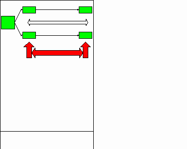
Relationship between sample & population

Sadly this file has converted very badly to GIF format. It shows the relationships between observations (single woman on left!), samples (gaggle in middle) made up of observations and, at least in theory,
drawn at random from population (e.g. British adults!)
Sample parameters and population parameters
- Samples give you data
- Descriptive sample statistics summarise those data... e.g.
...
- rate (for binary variables)
- mean
- median, quartiles & centiles
- standard deviation & deviance
- Two groups of statistics:
- "central tendency" or "location"
- scatter about that central tendency
Sampling and confidence intervals
- you have a sample parameter (typically a mean or a rate)
- this is a "best guess" estimate of the population
parameter
- sample size determines how precisely you estimate the "true"
value for the population
- larger sample => greater precision
- confidence intervals indicate precision
N.B. difference between C.I. and variance or s.d.:
(that the s.d. is a description of scatter of observations in
the sample, whereas the C.I. is an estimate of the location
of a parameter in the population from which the sample
was taken)
n=100    mean = 15.5    s.d. = 5.1    95%CI = 14.5 to 16.5
n=1000   mean = 15.5    s.d. = 5.1    95%CI = 15.2 to 15.8
n=10000  mean = 15.5    s.d. = 5.1    95%CI = 15.4 to 15.6
Confidence intervals continued
- 95% confidence interval will span the "true" population
value of the parameter in 95% of experiments provided ...
- ... that the assumptions underlying the calculation are correct
- not possible to say for any 95% C.I. that it contains
the "true" population value
95% C.I. for sample rate of .1
      n      95% C.I.
     10    .0025 to .45
     20    .012  to .32
     40    .028  to .24
     50    .033  to .22
     70    .041  to .20
    100    .049  to .18
    200    .062  to .15
    500    .075  to .13
  1,000    .082  to .12
  5,000    .092  to .11
 10,000    .094  to .11
100,000    .098  to .102
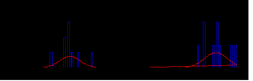
95% C.I. for sample rate of .1

This should show the last set of figures as a plot. The axes have been completely lost in translation but I hope it still gives
a flavour of the narrowing of the 95% confidence interval as the sample size increases (from Left to Right).
95% C.I. for a mean - simulation of a classical psychopharmacology
study ("experiment")
This converted even less satisfactorily than the last two graphics. This shows how the pool of depressed subjects are split into two samples
(by randomisation), their depression scores are noted, then, double-blind, one group get active compound and the other
placebo for a suitable period after which their depression scores are again noted. The dependent variable to be analysed
will be the difference between the two scores so a negative will indicate success: a reduction in depression.
Simulation of a two group comparison study
- measure of interest is four week drop in HRSD rating
- equal sized groups (not paired)
- independent observations
- advantage to active compound: -5
- both groups equal s.d. 7
- 200 such studies simulated for ...
n = 10
This has converted so badly it seems scarcely worth the candle. It is supposed to show
two samples each of n=10 one with a group of drops representing the
active compound, the other the placebo where the samples were made on the
assumptions shown in the definition above. This particular
run of the simulation gives rise to the 95% confidence intervals below.
- Active compound: -26.0 to -18.0
- Placebo: -15.0 to -7.0
- Difference: -16.6 to -6.0
30 simulations
n = 10

This shows a the confidence intervals for a number of runs of the simulation.
n = 100
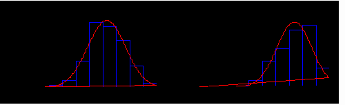
Another terrible conversion. It shows the two samples now with n=100
but still with the same population model. This run of the simulation
gives rise to the 95% confidence intervals below.
- Active compound: -20.0 to -17.3
- Placebo: -14.3 to -11.8
- Difference: -7.5 to -3.8
30 simulations
n = 100

Confidence intervals and their assumptions
Confidence intervals are calculated on a model of the study
with assumptions
- for rates these assumptions are:
- random sampling from large (infinite) population(s)
- independent observations
- constant probabilities within each group
- for means these assumptions are (for pt.II):
- random sampling from large (infinite) populaton(s)
- independent observations
- Normal or Gaussian distributions
- equal population variance within each group
(for C.I. of difference between independent groups)
Erotomania & the erotic, delusional transference
- delusions are falsely derived, unshakeable beliefs
- the content of an erotic transference (and erotomania) is
apparently libidinal, sexual love
- ... but is often the cover for envy and hatred
- psychiatry has just such a relationship with statistical tests
and the p value
- ... not that they're not great in a reality oriented relationship!
Inferential statistics "hypothesis testing", "tests"
- this branch of statistics is:
- clear
- rigorous
- objective
- potentially enlightening
- dichotomous
- it is not:
- a means of transmuting uncertainty to certainty
- immune to abuse
- complete and balanced (as it's usually (ab)used)
Assumptions underpinnning inferential statistics
Test the probability of getting results as interesting as
you did given:
- "null" hypothesis
- random sampling from large (infinite) population
- independent observations
- other assumptions if dealing with means not rates
If this is less than a certain level (chosen in advance) ...
... the result is declared "significant"
- the pre chosen level is the alpha or "type I error
rate"
... i.e. the probability of deciding that an effect is "significant"
given that the null hypothesis were true for the population
The meaning of "significant" or "p <
.05"
The probability of a result as marked as this was lower than
1 in 20 if the null hypothesis (and other assumptions) were true
- this doesn't mean:
- it's clinically interesting
- it's managerially interesting
- it's theoretically or philosophically interesting
- you can say anything for certain about your next patient
- however it is:
- a completely logical way to decide significance in terms of
likelihoods
- and other ways of doing this are even more complex
and contentious!
Null hypotheses
- Remember "statisticians do it backwards
(but beautifully)"
- therefore the null hypothesis is (depending on the test) that:
- the population mean is zero
- the population change is zero
- the difference between the population means is zero
- there is no association (no correlation) in the population
- it is a model of the population not the sample
- it's part of a set of assumptions forming a model that can
be tested against the sample data
So what's an "alternative hypothesis"?
- The alternative hypothesis is the logical complement to the
null hypothesis
- ... that there is
- a population mean other than zero
- population change other than zero
- a difference between population means other than zero
- an association (correlation) in the population that is other
than zero
- whereas there is only one quantitative null hypothesis
....
- ... there are many possible quantitative alternative hypotheses
contained within the one logical alternative hypothesis
Alternative hypotheses, type II error rates and statistical
power
- There is one type I error rate for a study
- but there are an infinite no. of possible type II error rates
- ... the risk of deciding "non-significant"
- ... when the null hypothesis was not true
- ... for each of the infinite number of true population effects
Given a small study and/or a weak "true" population
effect the type II error rate is often very high (.9 for many
published "NS" results)
- i.e. a non-significant result does not prove there is no population
effect
Statistical power
Statistical power is the probability
- given a certain "true" population effect
- and all the other assumptions of the test
- that you would have found a significant result
- given your sample size(s)
Statistical power is:
- (1 - type II error rate)
- or (1 - beta)
As statistical power has generally been neglected, confidence
intervals are replacing p values as they show how large
an effect you could be missing
Confidence intervals and "significance" testing
Historically two very different approaches to the problem and
there was much acrimonious argument between protagonists of the
two approaches
- but generally mathematically complementary
- as a 95% confidence interval that doesn't embrace a zero effect
is equivalent to a significant effect
- ... when the assumptions are the same (true for most tests
on means)
Research frames likely in the exam
- One study group (and one measure)
- One study group (and two measures)
- how much associated/correlated?
- Differences between groups (one measure)
- The remainder: "multivariate statistics"
A linked set of questions
"How many psychiatric registrars are depressed?"
- Prevalence
- always think of as a ratio:
number affected
number at risk
- point prevalence
- period prevalence
- Incidence
- always a ratio but now of onsets
number of new cases (or relapses)
number at risk
Quality of measurement - 1 scaling
- nominal scaling
- ordinal scaling
- interval scaling
- ratio scaling
(N.B. Binary measurements are not easy to classify)
Quality of measurement - 2
Qualities of a binary measure of caseness
qualities that are independent of prevalence
more clinically useful qualities that are dependent on prevalence
- positive predictive value
- negative predictive value
indications of lack of contamination
The four screening numbers: a,b,c,d
| "True" status | | Score on test | |
| -ve | +ve | total |
| non-case | a | b | a+b |
| case | c | d | c+d |
| total | a+c | b+d | a+b+c+d = n
|
          a = true negatives               b = false positives
          c = false negatives              d = true positives
sensitivity = d/(c+d)            specificity = a/(a+b)
        PPV = d/(b+d)                    NPV = a/(a+c)


PPV = "Positive predictive value", probability a positive test result will be a case
NPV = "Negative predictive value", probability a negative test result will be a non-case
Reliability
Evidence that the measure is not contaminated by random variation
- stability across time (if the latent variable is supposed
to be stable)
- "test-retest reliability"
- stability across observers
- "inter-rater reliability"
- stability across subunits of the measure
- "internal reliability"
Validity
- Evidence of criterion related validity
- concurrent validity
- predictive validity
- Evidence of content validity
- assumes you have definite agreement about content
- includes "face validity"
- Evidence of construct validity
- is it located within a theoretical model ...
- ... aspects of which can be measured ...
- ... and do the measurements fit the theoretical model?
The "multiple tests" issue
- If the null hypothesis is true and you do:
- one test: type I error rate is a .05
- two tests: rate is 1 - (1- a)2 .098
- three tests: rate is 1 - (1- a)3 .143
- five tests: rate is 1 - (1- a)5 .226
- ten tests: rate is 1 - (1- a)10 .401
- twenty tests: rate is 1 - (1- a)20 .642
- thirty tests: rate is 1 - (1- a)30 .785
- fifty tests: rate is 1 - (1- a)50 .923
- ... so just don't tell the reader about the the non-significant
tests you conducted!
Distributional assumptions
For M.R.C.Psych. purposes there are two different classes
of statistical test
- those involving distributional assumptions, a.k.a. "parametric"
tests and based on Normal or Gaussian distributions
- those not involving distributional assumptions, a.k.a. "nonparametric",
applying automatically to counts & rates, or based on converting
scores to ranks
Parametric vs. non-parametric
- Parametric tests give better statistical power than non-parametric
for similar sample sizes
- but non-parametric tests not dependent on distributional assumptions
- choice between the two best taken after consultation with
expert statistician
Matching "tests" to problems
- If it's a count, apply Chi squared test
- paired tests:
- if it's roughly Gaussian, apply paired t-test
- if not, Wilcoxon test
- unpaired tests of difference between two groups
- Gaussian and similar variances in each group (or similar sample
sizes) - unpaired t-test (or ANOVA)
- if not, Mann-Whitney test
- tests of differences between >2 groups
- Gaussian ... - ANOVA
- if not, Kruskal-Wallis test
Matching "tests" to problems (contd.)
- if it's an association or correlation
- between counts - Chi squared and related phi
- ... or Kappa (particularly for looking at inter-rater
agreement)
- between Gaussian variables (similar variances not necessary)
- Pearson correlation coefficient
between non-Gaussian variables - Spearman or Kendall correlation
coefficients (latter better if many ties which is often the case
on short ordinal ratings)
"Robustness" of statistical tests
- There are two main distributional assumptions:
- Gaussian shape
- with the same variance in each group (for >1 group)
parametric tests are often robust (i.e. continue to give about
the right type I and II error rates) for distributions that are
only roughly Gaussian
- many things can be transformed to "roughly" Gaussian
e.g. by taking logs (pH is one example)
- parametric test are also often robust to differing variances
provided sample sizes in the groups are similar
Multivariate statistics
The one fairly unproblematical one is internal reliability (coefficient
alpha): the proportion of common variance in a set of items
- Others are:
- factor analysis
- cluster analysis
- multivariate ANOVA (MANOVA)
- problems are:
- need large sample sizes
- not as robust to distribution as univariate statistics
- they're complex, easy to "blind with science"!