Show code
### this is just the code that creates the "copy to clipboard" function in the code blocks
htmltools::tagList(
  xaringanExtra::use_clipboard(
    button_text = "<i class=\"fa fa-clone fa-2x\" style=\"color: #301e64\"></i>",
    success_text = "<i class=\"fa fa-check fa-2x\" style=\"color: #90BE6D\"></i>",
    error_text = "<i class=\"fa fa-times fa-2x\" style=\"color: #F94144\"></i>"
  ),
  rmarkdown::html_dependency_font_awesome()
)
Bootstrapping Spearman correlation coefficient
Traditionally people used the Spearman correlation coefficient where the sample observed distributions of the variables being correlated were clearly not Gaussian. The logic is that as the Spearman correlation is a measure of correlation between the ranks of the values, the distribution of the scores, population or sample, was irrelevant to any inferential interpretation of the Spearman correlation. By contrast, inference about the statistical (im)probability of a Pearson correlation, or a confidence interval (CI) around an observed correlation, was based on maths which assumed that population values were Gaussian. This is simply and irrevocably true: so if the distributions of your sample scores are way off Gaussian then the p values and CIs for a Pearson can be very misleading.
The logic of doing a test of fit to Gaussian on your sample data (univariate and/or bivariate test of fit) is dodgy as if your sample is small then even a large deviation from Gaussian that may give very poor p values and CIs has a fair risk of not being flagged as statistically significantly different from Gaussian and with a large sample, even trivial deviations from Gaussian that would have no effect on the p values and CIs will show as statistically significant. How severe that problem is should really have simulation exploration and I haven’t searched for that but the theoretical/logical problem is crystal clear.
Keen supporters of non-parametrical statistical methods sometimes argued, reasonably to my mind, that the simple answer was to use non-parametric tests regardless of sample distributions, their opponents argued that this threw away some statistical power: true but the loss wasn’t huge.
All this has been fairly much swept away, again, to my mind, by the arrival of bootstrapping which allows you, for anything above a very small sample and for pretty much all but very, very weird distributions, to get pretty robust CIs around observed Pearson correlations regardless of the distributions, population or sample distributions, of the variables.
Because of this I now report Pearson correlations with bootstrap CIs around them for any correlations unless there is something very weird about the data. This has all the advantages of CIs over p values and is robust to most distributions.
However, I often want to compare with historical findings (including my own!) that were reported using Spearman’s correlation so I still often report Spearman correlations. However, there is no simple parametric CI for the Spearman correlation and I’m not sure there should be outside the edge case where you have perfect ranking (i.e. no ties on either variable). Then the Spearman correlation is the Pearson correlation of the ranks and I think the approximation of using the parametric Pearson CI computation for the Spearman is probably sensible. I am not at all sure that once you have ties that you can apply the same logic though probably putting in n as the lower of the number of distinct values of the two variables probably gives a safe but often madly wide CI. (“Safe” in the sense that it will include the true population correlation 95% of the time (assuming that you are computing the usual 95% CI)).
Fortunately, I can see reason why the bootstrap cannot be used to find a CI around an observed Spearman correlation and this is what I do now when I am reporting a Spearman correlation.
Show code
getCISpearmanTxt <- function(x, bootReps = 999, conf = .95, digits = 2) {
  ### function to give bootstrap CI around bivariate Spearman rho
  ###  in format "rho (LCL to UCL)"
  ### expects input data in a two column matrix, data frame or tibble: x
  ### bootReps, surprise, surprise, sets the number of bootstrap replications
  ### conf sets the width of the confidence interval (.95 = 95%)
  ### digits sets the rounding
  require(boot) # need boot package!
  ### now we need a function that
  spearmanForBoot <- function(x,i) {
    ### function for use bootstrapping Spearman correlations
    cor(x[i, 1],
        x[i, 2],
        method = "spearman",
        use = "pairwise.complete.obs")
  }
  ### now use that to do the bootstrapping
  tmpBootRes <- boot(x, statistic = spearmanForBoot, R = bootReps)
  ### and now get the CI from that, I've used the percentile method
  tmpCI <- boot.ci(tmpBootRes, type = "perc", conf = conf)
  ### get observed Spearman correlation and confidence limits as vector
  retVal <- (c(tmpBootRes$t0,
           tmpCI$percent[4],
           tmpCI$percent[5]))
  ### round that
  retVal <- round(retVal, digits)
  ### return it as a single character variable
  retVal <- paste0(retVal[1],
                   " (",
                   retVal[2],
                   " to ",
                   retVal[3],
                   ")")
  retVal
}

getCISpearmanList <- function(x, bootReps = 999, conf = .95) {
  ### function to give bootstrap CI around bivariate Spearman rho
  ###  returns a list with items obsCorr, LCL and UCL
  ### expects input data in a two column matrix, data frame or tibble: x
  ### bootReps, surprise, surprise, sets the number of bootstrap replications
  ### conf sets the width of the confidence interval (.95 = 95%)
  require(boot) # need boot package!
  ### now we need a function that
  spearmanForBoot <- function(x,i) {
    ### function for use bootstrapping Spearman correlations
    cor(x[i,1],
        x[i,2],
        method = "spearman",
        use = "pairwise.complete.obs")
  }
  ### now use that to do the bootstrapping
  tmpBootRes <- boot(x, statistic = spearmanForBoot, R = bootReps)
  ### and now get the CI from that, I've used the percentile method
  tmpCI <- boot.ci(tmpBootRes, type = "perc", conf = conf)
  ### return observed Spearman correlation and confidence limits as a list
  retVal <- list(obsCorrSpear = as.numeric(tmpBootRes$t0),
                 LCLSpear = tmpCI$percent[4],
                 UCLSpear = tmpCI$percent[5])
  retVal
}

getCIPearsonTxt <- function(x, bootReps = 999, conf = .95, digits = 2) {
  ### function to give bootstrap CI around bivariate PearsonR
  ###  in format "R (LCL to UCL)"
  ### expects input data in a two column matrix, data frame or tibble: x
  ### bootReps, surprise, surprise, sets the number of bootstrap replications
  ### conf sets the width of the confidence interval (.95 = 95%)
  ### digits sets the rounding
  require(boot) # need boot package!
  ### now we need a function that
  pearsonForBoot <- function(x,i) {
    ### function for use bootstrapping Spearman correlations
    cor(x[i,1],
        x[i,2],
        method = "pearson",
        use = "pairwise.complete.obs")
  }
  ### now use that to do the bootstrapping
  tmpBootRes <- boot(x, statistic = pearsonForBoot, R = bootReps)
  ### and now get the CI from that, I've used the percentile method
  tmpCI <- boot.ci(tmpBootRes, type = "perc", conf = conf)
  ### get observed Spearman correlation and confidence limits as vector
  retVal <- (c(tmpBootRes$t0,
           tmpCI$percent[4],
           tmpCI$percent[5]))
  ### round that
  retVal <- round(retVal, digits)
  ### return it as a single character variable
  retVal <- paste0(retVal[1],
                   " (",
                   retVal[2],
                   " to ",
                   retVal[3],
                   ")")
  retVal
}

getCIPearsonList <- function(x, bootReps = 999, conf = .95) {
  ### function to give bootstrap CI around bivariate Spearman rho
  ###  returns a list with items obsCorr, LCL and UCL
  ### expects input data in a two column matrix, data frame or tibble: x
  ### bootReps, surprise, surprise, sets the number of bootstrap replications
  ### conf sets the width of the confidence interval (.95 = 95%)
  require(boot) # need boot package!
  ### now we need a function that
  pearsonForBoot <- function(x,i) {
    ### function for use bootstrapping Spearman correlations
    cor(x[i,1],
        x[i,2],
        method = "pearson",
        use = "pairwise.complete.obs")
  }
  ### now use that to do the bootstrapping
  tmpBootRes <- boot(x, statistic = pearsonForBoot, R = bootReps)
  ### and now get the CI from that, I've used the percentile method
  tmpCI <- boot.ci(tmpBootRes, type = "perc", conf = conf)
  ### return observed Spearman correlation and confidence limits as a list
  retVal <- list(obsCorrPears = as.numeric(tmpBootRes$t0),
                 LCLPears = tmpCI$percent[4],
                 UCLPears = tmpCI$percent[5])
  retVal
}
Show code
### generate some Gaussian and some non-Gaussian data
n <- 5000 # sample size
set.seed(12345) # get replicable results

as_tibble(list(x = rnorm(n),
               y = rnorm(n))) -> tibDat

tibDat %>%
  pivot_longer(cols = everything()) %>%
  summarise(absMinVal = abs(min(value))) %>%
  pull() -> varMinVal

tibDat %>%
  mutate(xSquared = x^2,
         ySquared = y^2,
         xLn = log(x + varMinVal + 0.2),
         yLn = log(y + varMinVal + 0.2),
         xInv = 1/(x + varMinVal + 0.1),
         yInv = 1/(y + varMinVal + 0.1)) -> tibDat

tibDat %>%
  pivot_longer(cols = everything()) -> tibDatLong

ggplot(data = tibDatLong,
       aes(x = value)) +
  facet_wrap(facets = vars(name),
             ncol = 2,
             scales = "free",
             dir = "v") +
  geom_histogram(bins = 100) +
  theme_bw()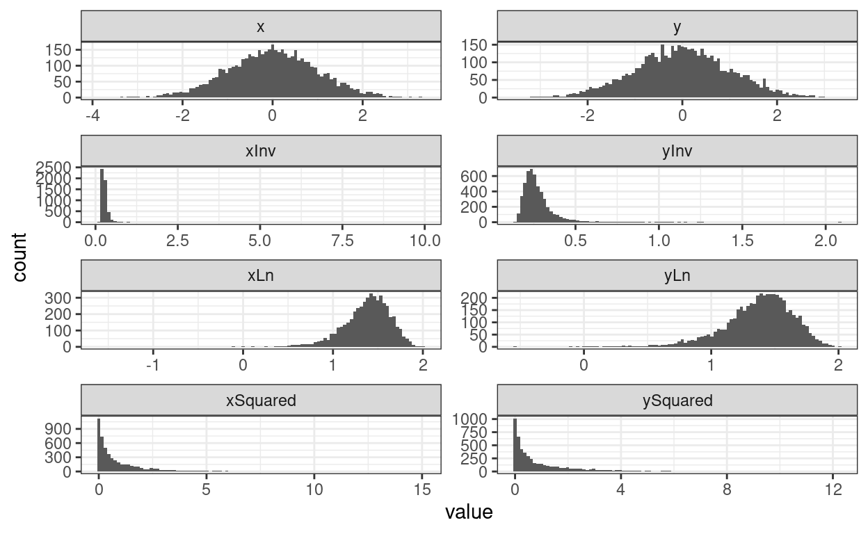
Show code
ggpairs(tibDat)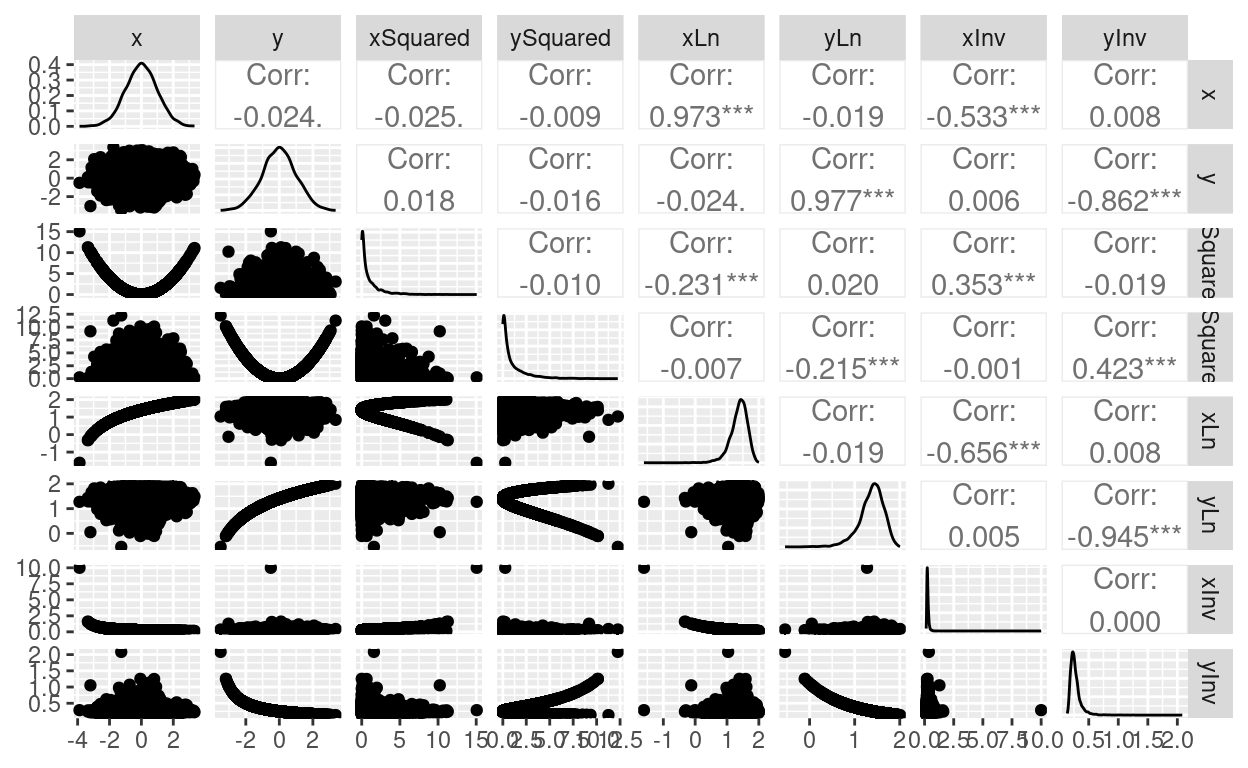
Good! Got some weird variables there: x and y are Gaussian random variables and uncorrelated then we have their squares, a natural log (after adding enough to the values to avoid trying to get ln(0)) and their inverses (with the same tweak to avoid getting 1/0).
Show code
options(dplyr.summarise.inform = FALSE)
tibDatLong %>%
  mutate(id = (1 + row_number()) %/% 2 ,
         var = str_sub(name, 1, 1),
         transform = str_sub(name, 2, 20),
         transform = if_else(transform == "", "none", transform),
         transform = ordered(transform,
                             levels = c("none", "Ln", "Inv", "Squared"),
                             labels = c("none", "Ln", "Inv", "Squared"))) %>%
  pivot_wider(id_cols = c(id, transform), values_from = value, names_from = var) -> tibDatLong2

tibDatLong2 %>%
  group_by(transform) %>%
  select(x, y) %>%
  summarise(corrS = list(getCISpearmanList(cur_data())),
            corrP = list(getCIPearsonList(cur_data()))) %>%
  unnest_wider(corrS) %>%
  unnest_wider(corrP) %>%
pander(justify = "lrrrrrr", split.tables = Inf)| transform | obsCorrSpear | LCLSpear | UCLSpear | obsCorrPears | LCLPears | UCLPears |
|---|---|---|---|---|---|---|
| none | -0.03547 | -0.06164 | -0.005442 | -0.02368 | -0.0495 | 0.003609 |
| Ln | -0.03547 | -0.06259 | -0.008897 | -0.01938 | -0.04774 | 0.01032 |
| Inv | -0.03547 | -0.06106 | -0.006073 | 0.0001815 | -0.0324 | 0.0382 |
| Squared | -0.00467 | -0.03253 | 0.02274 | -0.009833 | -0.03985 | 0.02017 |
That’s what we would expect to see: the observed Spearman correlations are the same for the raw data, the ln and inv transformed values (as these are transforms that preserve monotonic, i.e. ranked, ordered, relationships between values while changing the values a lot) but the value is different for the squared transform as that’s not monotonic. The values for the Pearson correlations change with ln and inv transforming as they should as the correlations between the transformed values are not the same as between the raw values. The CIs for the Spearman raw and ln and inv transformed values are not quite identical because the bootstrapping will have produced different bootstrapped samples for each. (I think there’s a way I could have got all three in the same call to boot() but that would have needed a different function to bootstrap.)
Reassuring that all the CIs include zero: you’d hope so really with n = 5000 and uncorrelated raw values.
Now let’s get a moderately correlated pair of variables.
Show code
### generate some Gaussian and some non-Gaussian data
n <- 5000 # sample size
set.seed(12345) # get replicable results

tibDat %>%
  mutate(y = x + y) %>%
  select(x, y) -> tibDat

tibDat %>%
  pivot_longer(cols = everything()) %>%
  summarise(absMinVal = abs(min(value))) %>%
  pull() -> varMinVal

tibDat %>%
  mutate(xSquared = x^2,
         ySquared = y^2,
         xLn = log(x + varMinVal + 0.2),
         yLn = log(y + varMinVal + 0.2),
         xInv = 1/(x + varMinVal + 0.1),
         yInv = 1/(y + varMinVal + 0.1)) -> tibDat

tibDat %>%
  pivot_longer(cols = everything()) -> tibDatLong

ggplot(data = tibDatLong,
       aes(x = value)) +
  facet_wrap(facets = vars(name),
             ncol = 2,
             scales = "free",
             dir = "v") +
  geom_histogram(bins = 100) +
  theme_bw()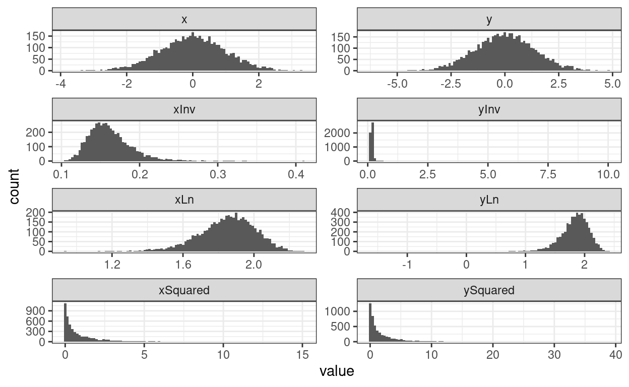
Show code
ggpairs(tibDat)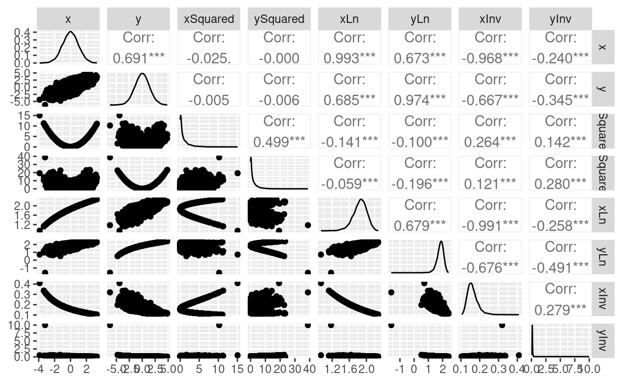
Show code
options(dplyr.summarise.inform = FALSE)
tibDatLong %>%
  mutate(id = (1 + row_number()) %/% 2 ,
         var = str_sub(name, 1, 1),
         transform = str_sub(name, 2, 20),
         transform = if_else(transform == "", "none", transform),
         transform = ordered(transform,
                             levels = c("none", "Ln", "Inv", "Squared"),
                             labels = c("none", "Ln", "Inv", "Squared"))) %>%
  pivot_wider(id_cols = c(id, transform), values_from = value, names_from = var) -> tibDatLong2

tibDatLong2 %>%
  group_by(transform) %>%
  select(x, y) %>%
  summarise(corrS = list(getCISpearmanList(cur_data())),
            corrP = list(getCIPearsonList(cur_data()))) %>%
  unnest_wider(corrS) %>%
  unnest_wider(corrP) %>%
pander(justify = "lrrrrrr", split.tables = Inf)| transform | obsCorrSpear | LCLSpear | UCLSpear | obsCorrPears | LCLPears | UCLPears |
|---|---|---|---|---|---|---|
| none | 0.666 | 0.6485 | 0.6833 | 0.6906 | 0.6755 | 0.7049 |
| Ln | 0.666 | 0.6496 | 0.683 | 0.679 | 0.6625 | 0.6956 |
| Inv | 0.666 | 0.6488 | 0.6823 | 0.279 | 0.2516 | 0.6728 |
| Squared | 0.3559 | 0.3311 | 0.3815 | 0.4992 | 0.4617 | 0.5347 |
web page counter