Subscale/total correlations

A look at subscale/total correlations in the null model

Show code

### this is just the code that creates the "copy to clipboard" function in the code blocks
htmltools::tagList(
  xaringanExtra::use_clipboard(
    button_text = "<i class=\"fa fa-clone fa-2x\" style=\"color: #301e64\"></i>",
    success_text = "<i class=\"fa fa-check fa-2x\" style=\"color: #90BE6D\"></i>",
    error_text = "<i class=\"fa fa-times fa-2x\" style=\"color: #F94144\"></i>"
  ),
  rmarkdown::html_dependency_font_awesome()
)

This came about from some work I am doing with colleagues looking at Authenticity Scale (AS; Wood et al., -Wood et al. (2008)). The AS has twelve items and a nicely balanced set of three subscales of four items each. The subscales are named Self-Alienation (SA), Accepting External Influence (AEI) and Authentic Living (AL). I was doing what I have always done before and looking at the simple correlations between the subscales and between them and the total score. As it happened a low correlation between one subscale and the other two took me back to something that has been in my mind a lot this year: when is a correlation structure that is not simply unidimensional/unifactorial, perhaps even fairly cleanly of two factors such that we shouldn’t report total scores but only the subscale (factor) scores?

That’s for another day and another blog post or several but I found myself aware that in a true null model in which correlations between the items of a measure are purely random, the correlations between subscale scores and the total score must be higher than zero as there is shared variance between the subscale score and the total score. That got me pondering why tradition has it (and like a slave, I have always followed it) that for subscale/total correlations we report the raw correlation but when looking item/total correlations we report “corrected” item/total correlations (CITCs), i.e. the correlation between the scores on the item and the scores on the whole scale corrected: with that item’s scores omitted.

If the items scores are Gaussian and uncorrelated and all have equal variance then it’s not rocket science to work out that the asymptotic Pearson correlation (i.e. the correlation as the sample size tends to \(\infty\)) between the subscale score and the total score will be:

\[ \sqrt{\frac{k_{subscale}}{k_{total}}} \]

Where \(k_{subscale}\) is the number of items in the subscale and \(k_{total}\) is the number of items in the entire measure. (Quick reductio ad absurdum checking: if \(k_{subscale}\) is zero then the correlation will be zero and if \(k_{subscale}\) is the same as \(k_{total}\)) then the correlation is one.)

So for the AS with four items per subscale the asymptotic correlation would be \(\sqrt{\frac{4}{12}}\), i.e. sqrt(1/3) = 0.577 (to 3 d.p.) were there no systematic covariance across the items.

Here’s the relationship between the correlation and the fraction of the total number of items in the subscale (always assuming a null model that there is no covariance across the items). I have added reference lines for the proportions of items in the subscales of the CORE-OM and the AS assuming their were zero population item covariance.

Show code

library(tidyverse)
valK <- 340
0:340 %>%
  as_tibble() %>%
  rename(fraction = value) %>%
  mutate(fraction = fraction / valK,
         R = sqrt(fraction)) -> tibRvals

tibble(scale = c("CORE-OM WB (4/34)",
                 "CORE-OM Risk (6/34)",
                 "CORE-OM Problems or Functioning (17/34)",
                 "AS any subscale (4/12)"),
       fraction = c(4/34, 6/34, 18/34, 4/12)) %>%
  mutate(R = sqrt(fraction)) -> tibCOREandAS

ggplot(data = tibRvals,
       aes(x = fraction, y = R)) +
  geom_point() +
  geom_line() +
  geom_linerange(data = tibCOREandAS,
             aes(xmin = 0, xmax = fraction, y = R)) +
  geom_linerange(data = tibCOREandAS,
                 aes(x = fraction, ymin = 0, ymax = R)) +
  geom_text(data = tibCOREandAS,
             aes(x = 0, y = R + .015, label = scale),
             hjust = 0,
             size = 2.2) +
  xlab(bquote(k[subscale]/k[total])) +
  ylab("Asymptotic correlation") +
  ggtitle("Plot of asymptotic subscale/total correlation\nagainst proportion of total items in subscale") +
  scale_x_continuous(breaks = (0:10/10)) +
  theme_bw() +
  theme(plot.title = element_text(hjust = .5))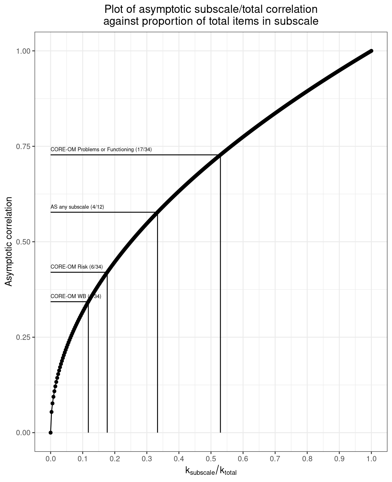

I amused myself simulating this for a sample size of 5000.

Show code

library(tidyverse)
options(dplyr.summarise.inform = FALSE)

### generate Gaussian null model data
set.seed(12345) # set for reproducible results
valN <- 5000 # sample size
valK <- 12 # total number of items

### now make up the data in long format, i.e.
###   an item score
###   an item label
###   a person ID
rnorm(valN * valK) %>% # gets uncorrelated Gaussian data
  as_tibble() %>%
  mutate(itemN = ((row_number() - 1) %% 12) + 1, # use modulo arithmetic to get item number
         item = str_c("I", sprintf("%02.0f", itemN)), # format it nicely
         ID = ((row_number() - 1) %/% 12) + 1, # use modulo arithmetic to get person ID 
         ID = sprintf("%03.0f", ID)) %>% # and format that, can now dump itemN
  select(-itemN) -> tibLongItemDat

### now just pivot that to get it into wide format, valK items per row
tibLongItemDat %>%
  pivot_wider(id_cols = ID, names_from = item, values_from = value) -> tibWideItemDat

### map items to scales (just sequentially here, that's not the AS mapping)
vecItemsScale1 <- str_c("I", sprintf("%02.0f", 1:4))
vecItemsScale2 <- str_c("I", sprintf("%02.0f", 5:8))
vecItemsScale3 <- str_c("I", sprintf("%02.0f", 9:12))

### now use those maps to get the subscale scores as well as the total score
tibWideItemDat %>%
  rowwise() %>%
  mutate(scoreAll = mean(c_across(-ID)),
         score1 = mean(c_across(all_of(vecItemsScale1))),
         score2 = mean(c_across(all_of(vecItemsScale2))),
         score3 = mean(c_across(all_of(vecItemsScale3)))) %>%
  ungroup() -> tibWideAllDat

tibWideAllDat %>%
  select(starts_with("score")) -> tibScores

### corrr::correlate() has a message about the method and handling of missing
### punches through markdown despite the block header having "message=FALSE"
### I could have wrapped this in suppressMessages() however you can suppress 
### that with "quiet = TRUE", see below
tibScores%>%
  ### here is the "quiet = TRUE" suppression of the message
  corrr::correlate(diagonal = 1, quiet = TRUE) %>%
  mutate(across(starts_with("score"), round, 2)) %>%
  pander::pander(justify = "lrrrr", digits = 2)

term	scoreAll	score1	score2	score3
scoreAll	1	0.57	0.58	0.59
score1	0.57	1	-0.01	0.01
score2	0.58	-0.01	1	0.01
score3	0.59	0.01	0.01	1

And here’s the plot of the simulated scores. The blue lines are the linear regression lines.

Show code

lm_fn <- function(data, mapping, ...){
  p <- ggplot(data = data, mapping = mapping) + 
    geom_point(alpha = .05) + 
    geom_smooth(method=lm, fill="blue", color="blue", ...)
  p
}


GGally::ggpairs(tibScores,
                lower = list(continuous = lm_fn)) +
  theme_bw()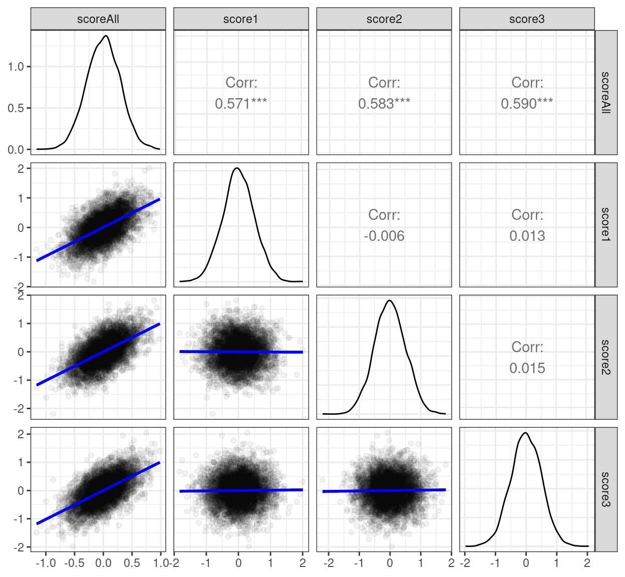

I am still not sure why we report CITCs for item analyses but raw subscale/total correlations for subscales. I keep trying to convince myself there’s a logic to my long entrenched behaviour but I’m not sure there is. I have a suspicion that we have all been doing it following others’ examples and that it started long ago when SPSS made CITCs easy to compute in its RELIABILITY function. I have long felt that RELIABILITY was one of the better parts of SPSS!

Visit count

free counter