Explanation
This file is simply a cumulative collection of code I wrote to create graphics (or occasionally raw numbers) for entries in the glossary for our book Outcome measures and evaluation in counselling and psychotherapy.
- Information about the book is at https://ombook.psyctc.org/SAGE/
- Supplementary information is at https://ombook.psyctc.org/book/ and …
- … the glossary itself is at https://ombook.psyctc.org/glossary/
I’m not claiming the code is good, some of it certainly isn’t, but it works. Some of it uses real data which for now I am not making available until I am sure that is safe and OK with others involved in collecting the data.
Show code
### this is just the code that creates the "copy to clipboard" function in the code blocks
htmltools::tagList(
  xaringanExtra::use_clipboard(
    button_text = "<i class=\"fa fa-clone fa-2x\" style=\"color: #301e64\"></i>",
    success_text = "<i class=\"fa fa-check fa-2x\" style=\"color: #90BE6D\"></i>",
    error_text = "<i class=\"fa fa-times fa-2x\" style=\"color: #F94144\"></i>"
  ),
  rmarkdown::html_dependency_font_awesome()
)
Notes to self
- Best to store theme
- Always set xlab and ylab explicitly
- Using ggsave helps create standard size
- Probably correct not to bother with plot titles for simple plots
Show code
setwd("/media/chris/Clevo_SSD2/Data/MyR/R/distill_blog/test2/_posts/2021-11-09-ombookglossary")
library(tidyverse)
library(janitor)
library(pander)
library(CECPfuns)
library(flextable)

### set theme here
theme_set(theme_bw())
theme_update(plot.title = element_text(hjust = .5),
             plot.subtitle = element_text(hjust = .5),
             axis.title = element_text(size = 15))
Entries
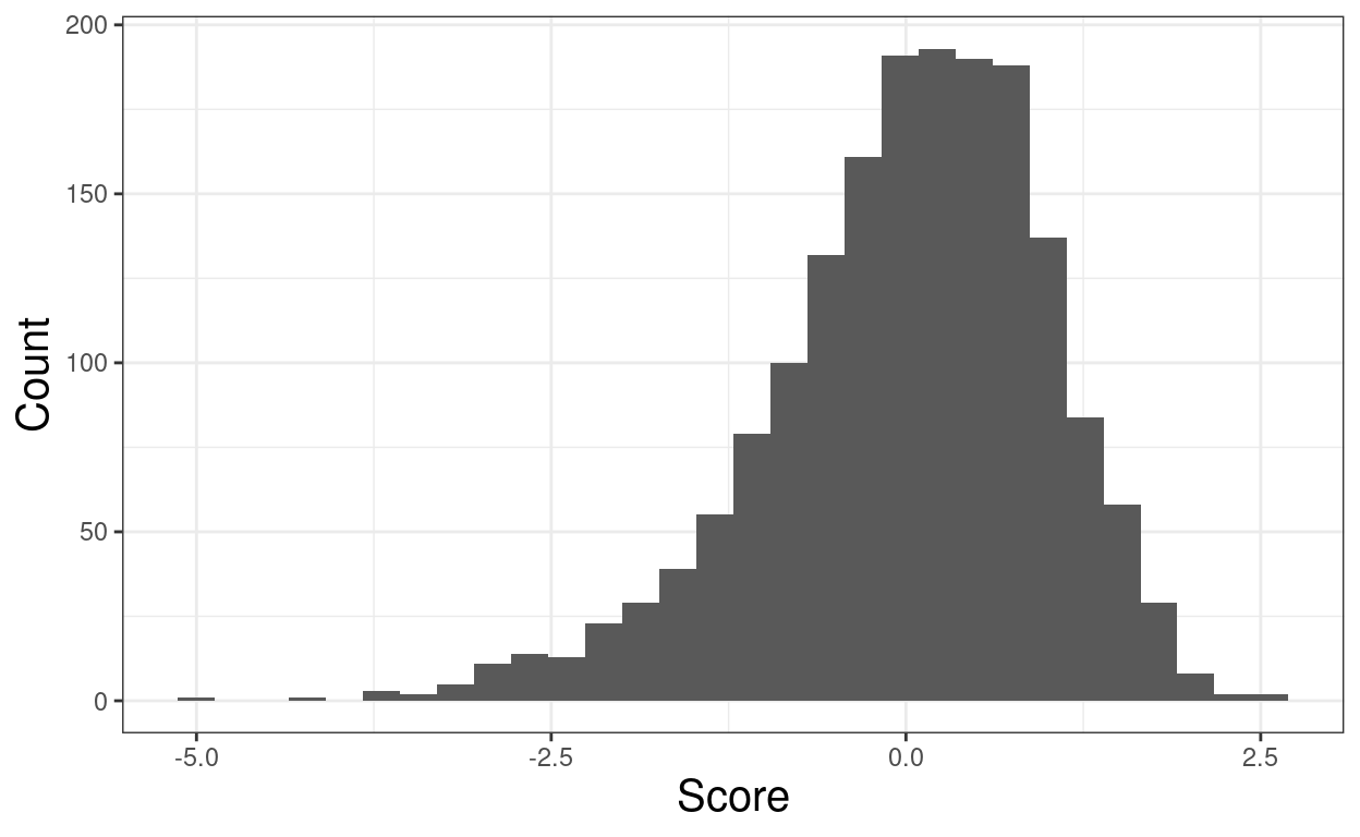
Illustrating mean and median from modified (truncated) Gaussian: pseudo CORE-OM “clinical” scores.
Show code
set.seed(12345)
valN <- 350
valMean <- 14
valMin <- 0
valMax <- 40
valSD <- 7

rnorm(valN, valMean, valSD) %>%
  as_tibble() %>%
  mutate(score = round(value),
         ### reset out of range scores
         score = if_else(score < 0, 0, score),
         score = if_else(score > 40, 40, score)) -> tibDat

tibDat %>%
  summarise(min = min(score),
            lQuart = quantile(score, .25),
            mean = mean(score),
            median = median(score),
            uQuart = quantile(score, .75),
            max = max(score),
            SD = sd(score)) -> tibSummary


ggplot(data = tibDat,
       aes(x = score)) +
  geom_histogram(center = TRUE) +
  geom_vline(xintercept = tibSummary$mean,
             colour = "blue",
             size = 2) +
    geom_vline(xintercept = tibSummary$median,
             colour = "green",
             size = 2) +
  scale_x_continuous(breaks = seq(0, 40, 2)) +
  xlab("Score") +
ylab("Count") 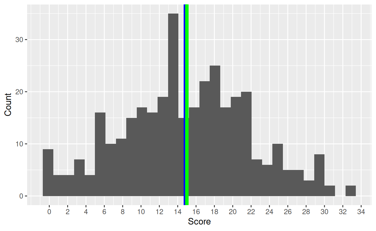
Show code
ggsave(filename = "mean.png",
       width = 1700,
       height = 1470,
       units = "px")
Now illustrate mean and median on positively skew data
Show code
[1] 767.6734Show code
mean(tibDat$score2)[1] 200.9804Show code
median(tibDat$score2)[1] 171.6222Show code
ggplot(data = tibDat,
       aes(x = score2)) +
  geom_histogram(center = TRUE) +
  geom_vline(xintercept = mean(tibDat$score2),
             colour = "blue",
             size = 2) +
  geom_vline(xintercept = median(tibDat$score2),
             colour = "green",
             size = 2) +
  scale_x_continuous(breaks = seq(0, 800, 50)) +
  xlab("Score") +
ylab("Count") 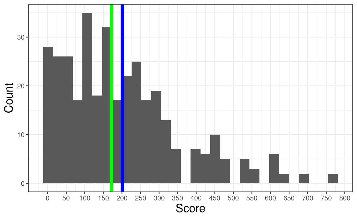
Show code
ggsave(filename = "mean2.png",
       width = 1700,
       height = 1470,
       units = "px")
Show code
Show code
ggsave(filename = "symm.png",
       width = 1700,
       height = 1470,
       units = "px")

standardiseVar <- function(x){
  x <- x - mean(x, na.rm = TRUE)
  x / sd(x, na.rm = TRUE)
}
tibSymm %>%
  mutate(score2 = (5 + score)^3,
         score2 = standardiseVar(score2)) -> tibPosSkew

ggplot(data = tibPosSkew,
       aes(x = score2)) +
  geom_histogram(center = TRUE) +
  xlab("Score") +
ylab("Count") 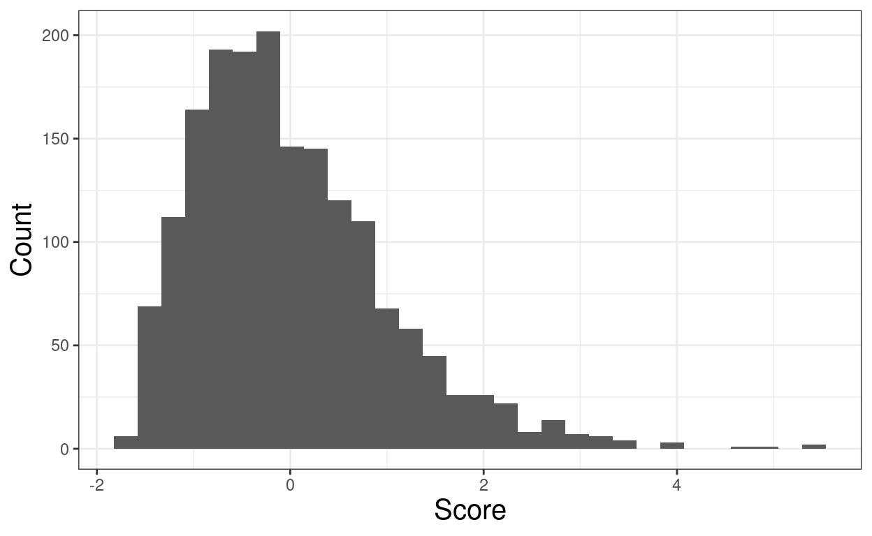
Show code
Show code
ggsave(filename = "negSkew.png",
       width = 1700,
       height = 1470,
       units = "px")
Illustrating quartiles and IQR
Show code
ggplot(data = tibDat,
       aes(x = score)) +
  geom_histogram(center = TRUE) +
  geom_vline(xintercept = tibSummary$mean,
             colour = "blue",
             size = 2) +
    geom_vline(xintercept = tibSummary$median,
             colour = "green",
             size = 2) +
  scale_x_continuous(breaks = seq(0, 40, 2)) +
  xlab("Score") +
ylab("Count") 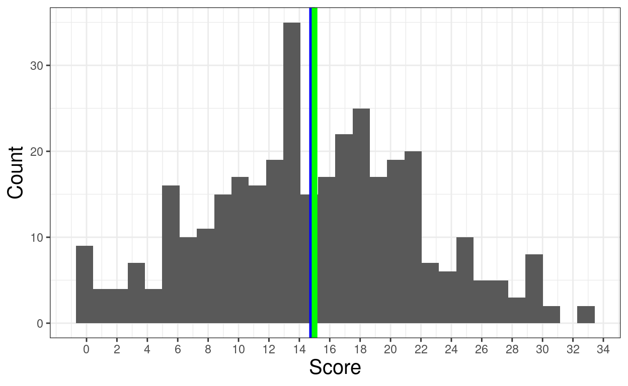
Show code
tibDat %>%
  rename(symm = score,
         skew = score2) %>%
  pivot_longer(cols = symm:skew, names_to = "dist", values_to = "score") -> tibDatLong

tibDatLong %>%
  group_by(dist) %>%
  summarise(min = min(score),
            lQuart = quantile(score, .25),
            mean = mean(score),
            median = median(score),
            uQuart = quantile(score, .75),
            max = max(score),
            SD = sd(score)) -> tibSummary2

tibSummary2 %>%
  select(dist, ends_with("Quart")) %>%
  pivot_longer(cols = ends_with("Quart")) -> tibIQR


ggplot(data = tibDatLong,
       aes(x = score)) +
  geom_histogram(center = TRUE) +
  geom_vline(data = tibSummary2,
             aes(xintercept = median),
             colour = "green",
             size = 2) +
  geom_vline(data = tibSummary2,
             aes(xintercept = mean),
             colour = "red",
             size = 1) +
  geom_vline(data = tibSummary2,
             aes(xintercept = lQuart),
             colour = "blue",
             size = 2) +
  geom_vline(data = tibSummary2,
             aes(xintercept = uQuart),
             colour = "blue",
             size = 2) +
  geom_line(data = tibIQR,
            aes(y = 5, x = value),
            arrow = arrow(ends = "both"),
            colour = "blue",
            size = 1.2) +
  facet_wrap(facets = vars(dist),
             nrow = 2,
             scales = "free") +
  xlab("Score") +
ylab("Count") 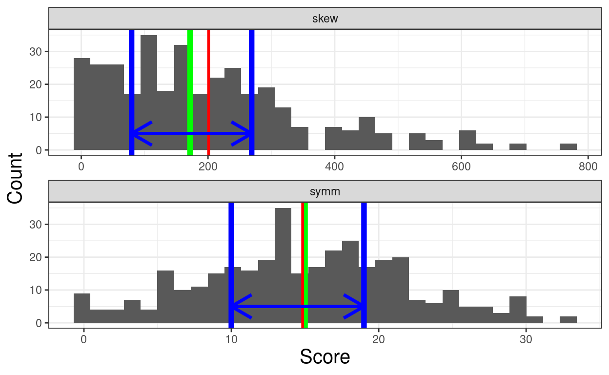
Show code
ggsave(filename = "IQR.png",
       width = 1700,
       height = 1470,
       units = "px")

tibSummary2 %>%
  filter(dist == "symm") -> tibSummary2symm
tibIQR %>%
  filter(dist == "symm") -> tibIQRsymm

ggplot(data = filter(tibDatLong, dist == "symm"),
       aes(x = score)) +
  geom_histogram(center = TRUE) +
  geom_vline(data = tibSummary2symm,
             aes(xintercept = median),
             colour = "green",
             size = 2) +
  geom_vline(data = tibSummary2symm,
             aes(xintercept = mean),
             colour = "red",
             size = 1) +
  geom_vline(data = tibSummary2symm,
             aes(xintercept = lQuart),
             colour = "blue",
             size = 2) +
  geom_vline(data = tibSummary2symm,
             aes(xintercept = uQuart),
             colour = "blue",
             size = 2) +
  geom_line(data = tibIQRsymm,
            aes(y = 5, x = value),
            arrow = arrow(ends = "both"),
            colour = "blue",
            size = 1.2) +
  xlab("Score") +
ylab("Count") 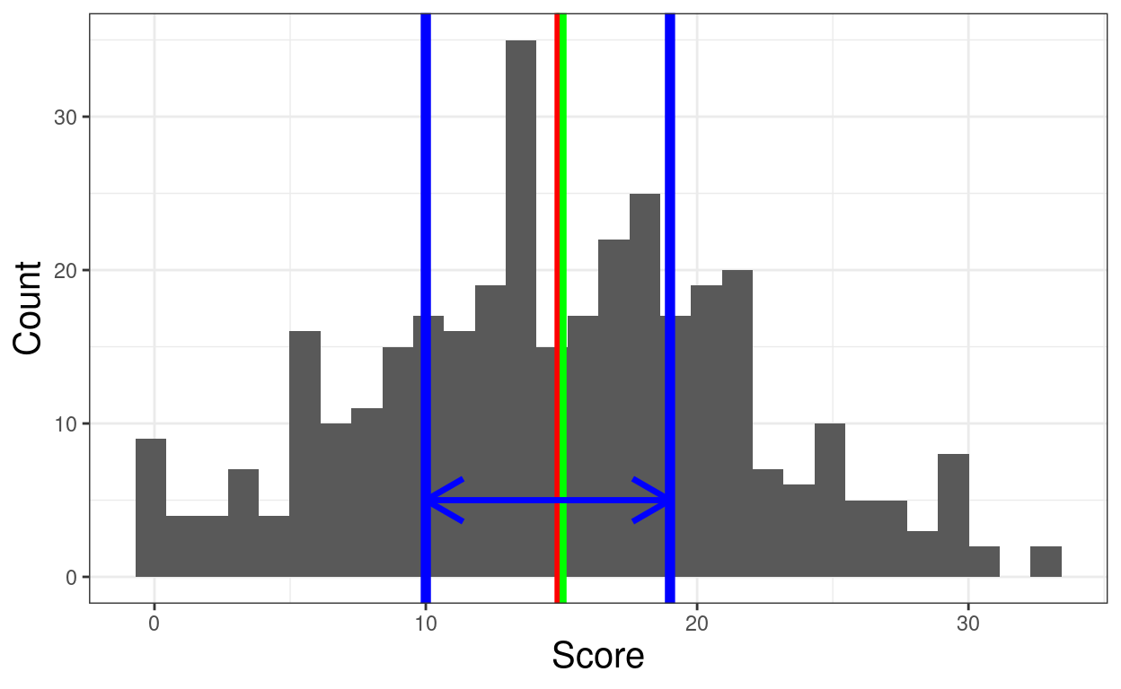
Show code
ggsave(filename = "IQRsymm.png",
       width = 1700,
       height = 1470,
       units = "px")


tibSummary2 %>%
  filter(dist == "skew") -> tibSummary2skew
tibIQR %>%
  filter(dist == "skew") -> tibIQRskew

ggplot(data = filter(tibDatLong, dist == "skew"),
       aes(x = score)) +
  geom_histogram(center = TRUE) +
  geom_vline(data = tibSummary2skew,
             aes(xintercept = median),
             colour = "green",
             size = 2) +
  geom_vline(data = tibSummary2skew,
             aes(xintercept = mean),
             colour = "red",
             size = 1) +
  geom_vline(data = tibSummary2skew,
             aes(xintercept = lQuart),
             colour = "blue",
             size = 2) +
  geom_vline(data = tibSummary2skew,
             aes(xintercept = uQuart),
             colour = "blue",
             size = 2) +
  geom_line(data = tibIQRskew,
            aes(y = 5, x = value),
            arrow = arrow(ends = "both"),
            colour = "blue",
            size = 1.2) +
  xlab("Score") +
ylab("Count") 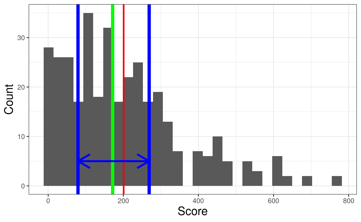
Show code
ggsave(filename = "IQRskew.png",
       width = 1700,
       height = 1470,
       units = "px")
More on quartiles
Show code
valN <- 300
set.seed(12345)

rnorm(valN, 40, 5) %>%
  as_tibble() %>%
  rename(score = value) -> tibDat1

ggplot(data = tibDat1,
       aes(x = score)) +
  geom_histogram(center = TRUE) +
  geom_vline(xintercept = mean(tibDat1$score),
             colour = "blue",
             size = 2) +
  geom_vline(xintercept = quantile(tibDat1$score, c(.25, .75)),
             colour = "green",
             size = 2) +
  xlab("Score") +
  ylab("Count") +
  scale_x_continuous(breaks = seq(0, 100, 10),
                     limits = c(0, 100))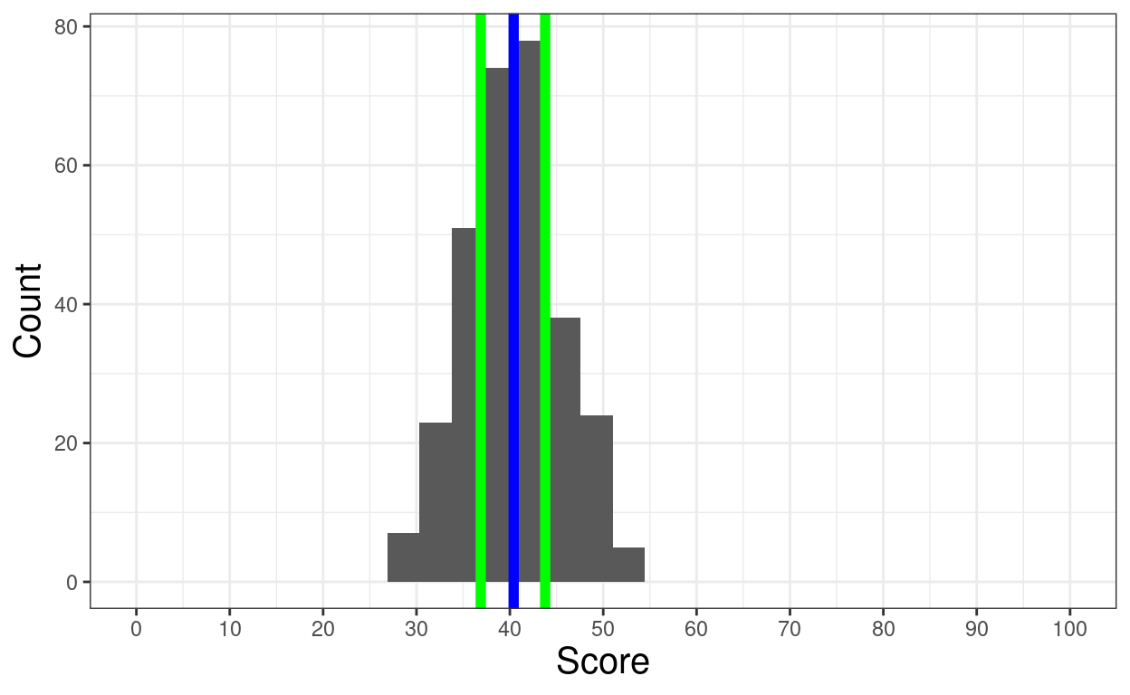
Show code
[1] 40.40703 25% 75%
36.87730 43.78248 Show code
rnorm(valN, 40, 15) %>%
  as_tibble() %>%
  rename(score = value) -> tibDat1

ggplot(data = tibDat1,
       aes(x = score)) +
  geom_histogram(center = TRUE) +
  geom_vline(xintercept = mean(tibDat1$score),
             colour = "blue",
             size = 2) +
  geom_vline(xintercept = quantile(tibDat1$score, c(.25, .75)),
             colour = "green",
             size = 2) +
  xlab("Score") +
  ylab("Count") +
  scale_x_continuous(breaks = seq(0, 100, 10),
                     limits = c(0, 100))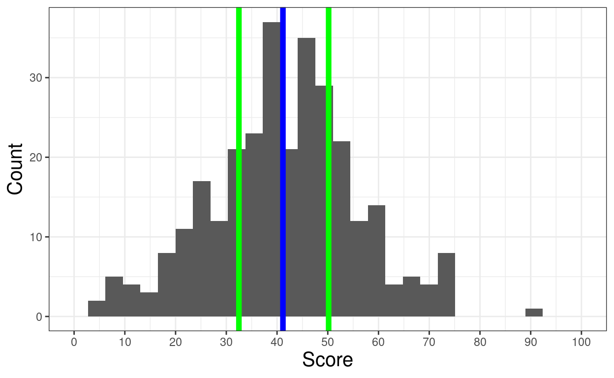
Show code
[1] 41.16123 25% 75%
32.48149 50.16902 Uniform distribution
Show code
set.seed(12345)
c(6, 6, 6, 6, 12, 18, 24, 50, 100, 200, 500, 1000, 1000, 5000, 10000) %>%
  as_tibble() %>%
  rename(sampSize = value) %>%
  mutate(sampID = row_number()) %>%
  # group_by(sampID) %>%
  # uncount(weights = sampSize, .id  = "indID")
  rowwise() %>%
  mutate(values = list(sample(1:6, sampSize, replace = TRUE))) %>%
  ungroup() %>%
  unnest_longer(values) -> tibUnif

# tibUnif

ggplot(data = filter(tibUnif, sampSize == 6),
       aes(x = values)) +
  # geom_histogram(binwidth = 1,
  #                boundary = 0) +
  geom_bar() +
  facet_grid(rows = vars(sampID),
             cols = NULL,
             scales = "free_y") +
  scale_y_continuous(breaks = 0:2) +
  scale_x_continuous(name = "Observed scores on each die", breaks = 1:6)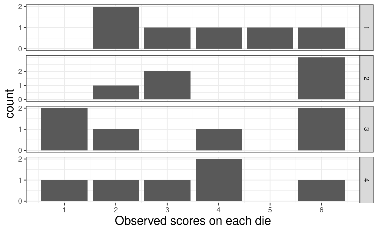
Show code
ggsave(filename = "dice1.png",
       width = 1700,
       height = 1470,
       units = "px")

tibUnif %>%
  filter(sampSize > 6 & sampSize < 200) -> tmpTib

ggplot(data = tmpTib,
       aes(x = values)) +
  geom_bar(aes(y = ..prop..)) +
  facet_grid(rows = vars(sampSize),
             cols = NULL,
             scales = "fixed") +
  scale_x_continuous(name = "Observed scores on each die", breaks = 1:6) +
  scale_y_continuous(name = "Proportion", breaks = (0:5)/10)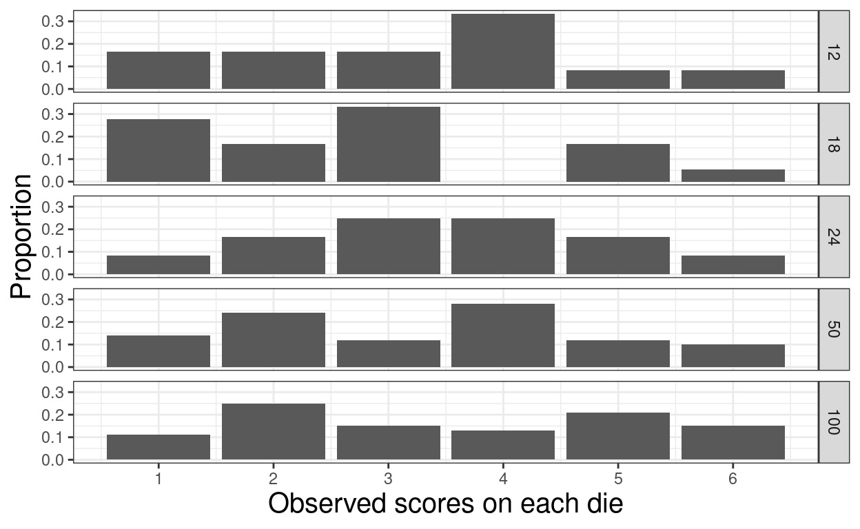
Show code
ggsave(filename = "dice2.png",
       width = 1700,
       height = 1470,
       units = "px")

tibUnif %>%
  filter(sampSize > 200) -> tmpTib

ggplot(data = tmpTib,
       aes(x = values)) +
  geom_bar(aes(y = ..prop..)) +
  facet_grid(rows = vars(sampSize),
             cols = NULL,
             scales = "fixed") +
  scale_x_continuous(name = "Observed scores on each die", breaks = 1:6) +
  scale_y_continuous(name = "Proportion", breaks = (0:5)/10)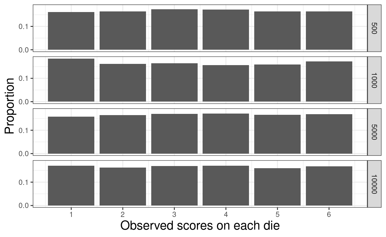
Show code
ggsave(filename = "dice3.png",
width = 1700,
height = 1470,
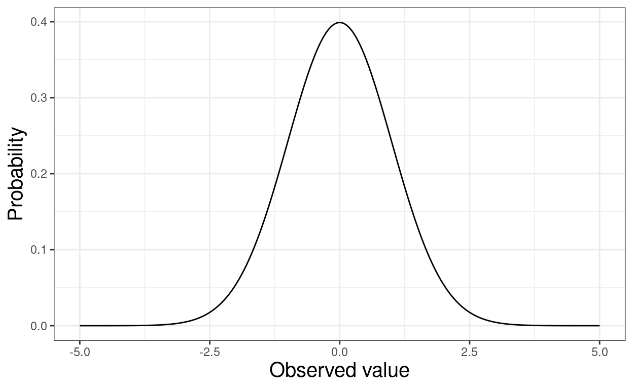
units = "px")Gaussian distribution
Throwing dice and central limit theorem
Show code
throwDice <- function(nThrows, nSides = 6, scoreSides = 1:6){
  ### function to simulate throwing dice (or anything really)
  ### defaults to six sided die with scores 1:6 but you can override that
  if(nThrows <= 0) {
    stop("nThrows must be positive")
  }
  if(nThrows > 8) {
    stop("nThrows must be under 9 (to keep things easy!)")
  }
  if(nThrows - round(nThrows) > .Machine$double.eps) {
    warning("nThrows wasn't integer, rounded to integer")
    nThrows <- round(nThrows)
  }
  newScores <- scoreSides
  while(nThrows > 1) {
    newScores <- as.vector(outer(newScores, scoreSides, FUN = "+"))
    nThrows <- nThrows - 1
  }
  newScores
}
# throwDice(0)
# throwDice(1)
# throwDice(1.1)
# throwDice(11)
# throwDice(2)
# length(throwDice(2))
# min(throwDice(2))
# max(throwDice(2))
# nThrows <- 3
# throwDice(nThrows)
# length(throwDice(nThrows))
# min(throwDice(nThrows))
# max(throwDice(nThrows))
# nThrows <- 4
# throwDice(nThrows)
# length(throwDice(nThrows))
# min(throwDice(nThrows))
# max(throwDice(nThrows))


1:8 %>%
  as_tibble() %>%
  rename(nThrows = value) %>%
  rowwise() %>%
  mutate(score = list(throwDice(nThrows)),
         nThrowsFac = factor(nThrows)) %>%
  ungroup() %>%
  unnest_longer(score) %>%
  group_by(nThrowsFac) %>%
  mutate(nScores = n()) %>%
  ungroup() %>%
  group_by(nThrowsFac, score) %>%
  summarise(nThrows = first(nThrows),
            nScores = first(nScores),
            n = n(),
            p = n / nScores) %>%
  ungroup() -> tibDiceThrows

ggplot(data = tibDiceThrows,
       aes(x = score, y = p, colour = nThrowsFac)) +
  geom_point()  +
  geom_line() +
  ylab("Probability") +
  scale_x_continuous(name = paste0("Total score from n dice (with n from 1 to ",
                                   max(tibDiceThrows$nThrows),
                                   ")"),
                     breaks = seq(2, max(tibDiceThrows$score), 2)) +
  scale_colour_discrete(name = "n(throws)") +
  theme(axis.text.x = element_text(angle = 70, hjust = 1))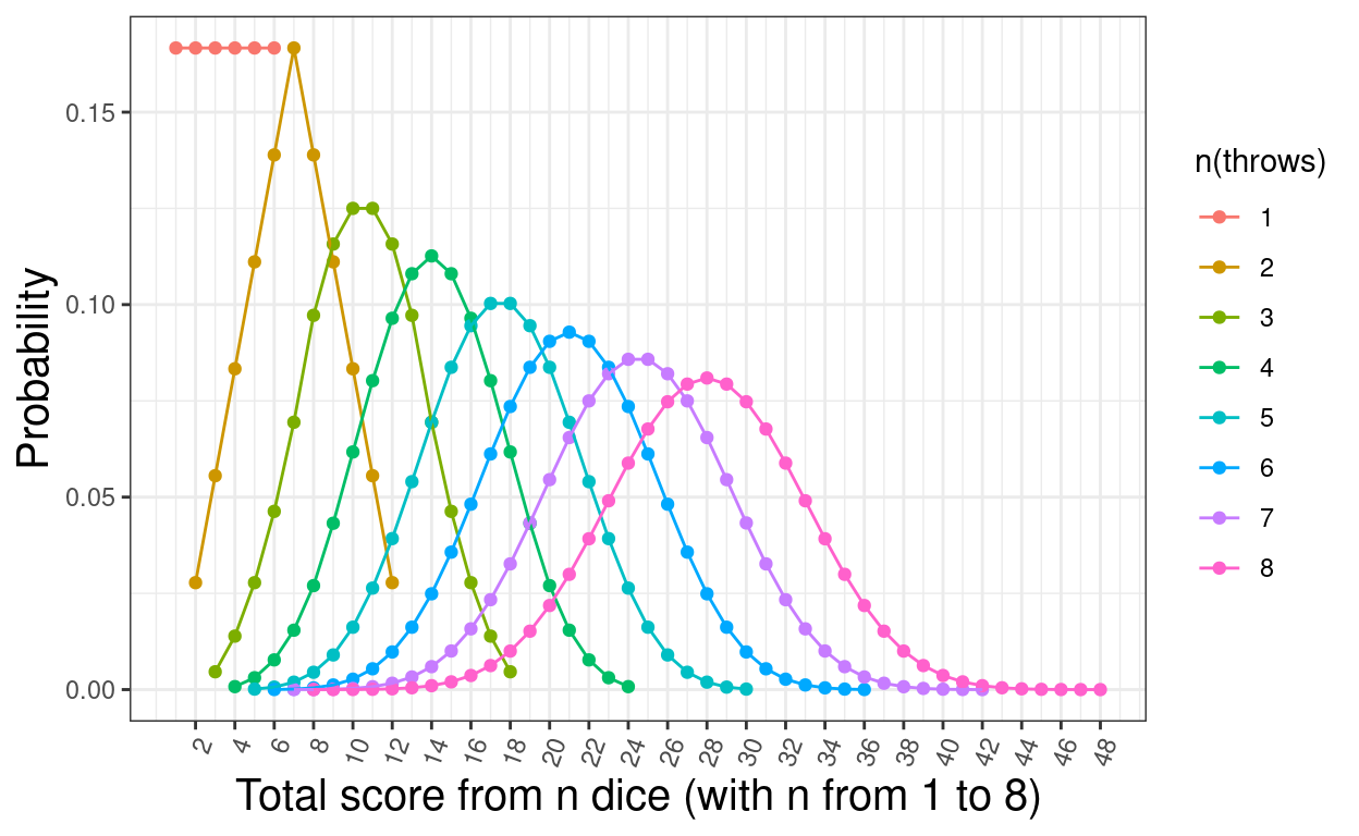
Show code
ggsave(filename = "throwingDice.png",
       width = 1700,
       height = 1470,
       units = "px")

tibDiceThrows %>%
  filter(nThrows == 6) -> tmpTib

tmpTib %>%
  summarise(n = n(),
            minScore = min(score),
            meanScore = Hmisc::wtd.mean(score, weights = nScores),
            maxScore = max(score),
            SDScore = sqrt(Hmisc::wtd.var(score, weights = nScores)),
            totP = sum(p)) -> tmpTibSumm

tmpTib %>%
  mutate(normScore = score - tmpTibSumm$meanScore,
         normScore = normScore / 3,
         normProb = dnorm(normScore) / 3) -> tmpTib
tmpTib %>%
  summarise(meanNormScore = mean(normScore),
            SDNormScore = sd(normScore),
            sumNormProb = sum(normProb))
# A tibble: 1 × 3
meanNormScore SDNormScore sumNormProb
<dbl> <dbl> <dbl>
1 0 3.03 1.00Show code
ggplot(data = tmpTib,
       aes(x = score, y = p)) +
  geom_point()  +
  geom_line() +
  ylab("Probability") +
  scale_x_continuous(name = "Total score from 6 dice",
                     breaks = 6:36)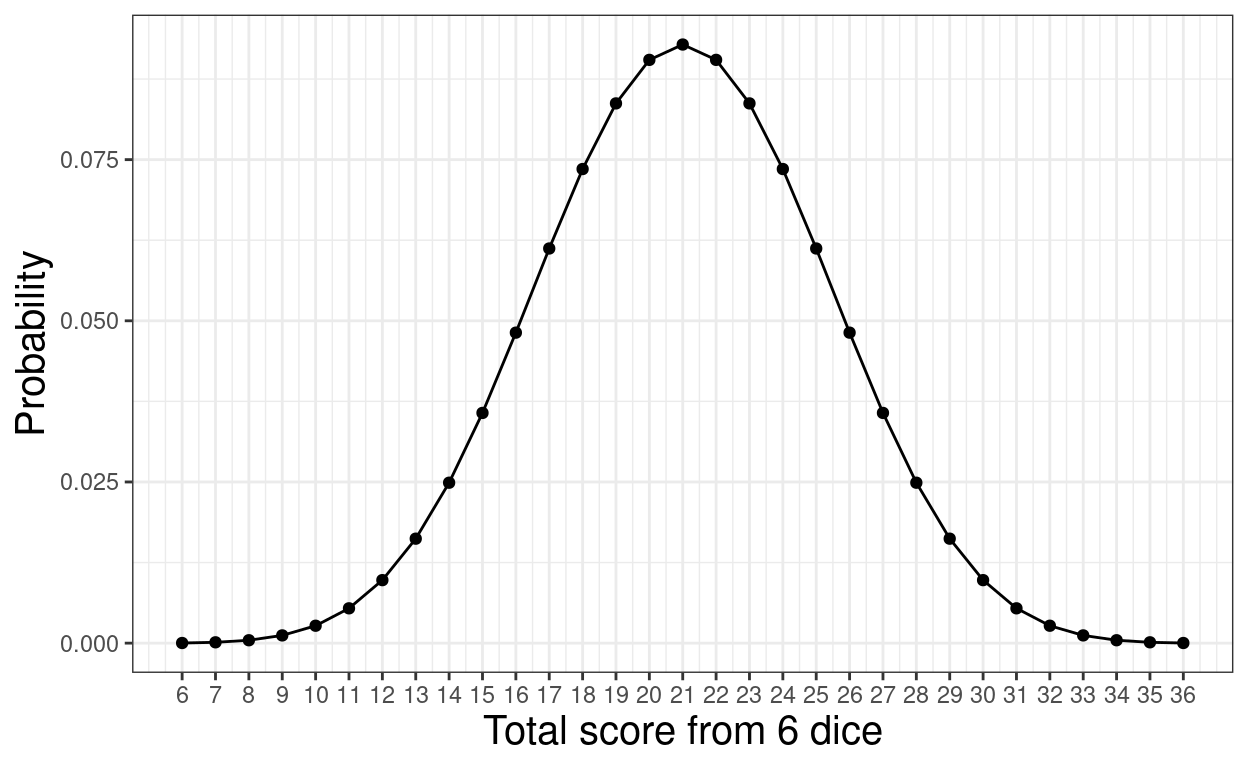
Show code
ggsave(filename = "throwing6Dice.png",
       width = 1700,
       height = 1470,
       units = "px")


ggplot(data = tmpTib,
       aes(x = score, y = p)) +
  geom_point()  +
  geom_line() +
  geom_point(aes(y = normProb),
            colour = "green") +
  geom_line(aes(y = normProb),
            colour = "green") +
  ylab("Probability") +
  scale_x_continuous(name = "Total score from 6 dice",
                     breaks = 2:max(tmpTib$score)) +
  scale_colour_discrete(name = "n(throws)")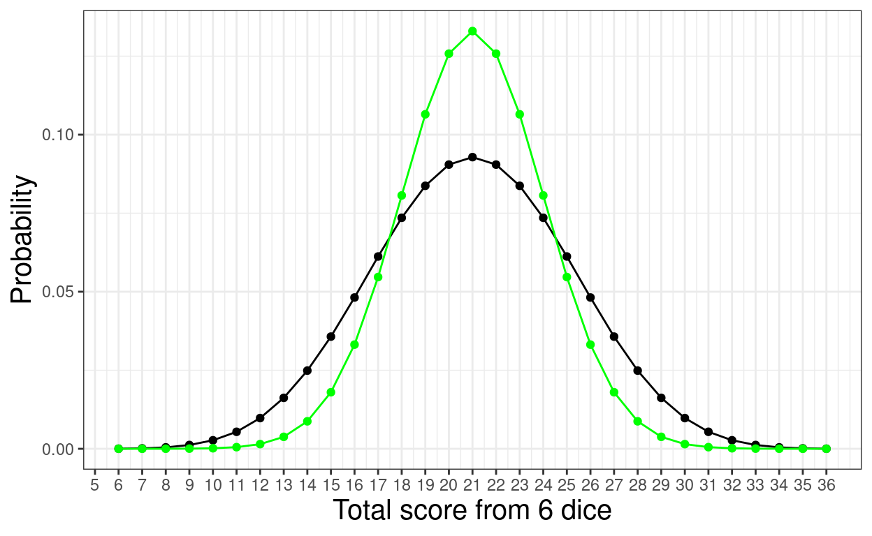
Show code
ggsave(filename = "throwing6DiceWithGaussian.png",
       width = 1700,
       height = 1470,
       units = "px")


ggplot(data = tmpTib,
       aes(x = score, y = p)) +
  geom_point()  +
  geom_line() +
  ylab("Probability") +
  scale_x_continuous(name = "Total score from 6 dice",
                     breaks = 2:max(tmpTib$score)) +
  scale_colour_discrete(name = "n(throws)")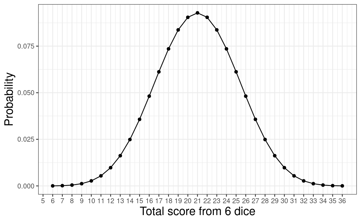
Show code
ggsave(filename = "throwing6Dice.png",
       width = 1700,
       height = 1470,
       units = "px")
Tossing coins and the central limit theorem
Show code
set.seed(12345)
nReps <- 50000
c(1:5, seq(10, 50, 10), 100, 200, 300, 400, 500) %>%
  as_tibble() %>%
  rename(nThrows = value) %>%
  rowwise() %>%
  mutate(score = list(rbinom(nReps, nThrows, .5))) %>%
  ungroup() %>%
  unnest_longer(score) %>%
  group_by(nThrows, score) %>%
  summarise(n = n(),
            p = n / nReps,
            nThrowsFac = factor(nThrows)) %>%
  ungroup() %>%
  group_by(nThrows) %>%
  mutate(scaledScore = scale(score)) -> tibBinom


ggplot(data = tibBinom,
       aes(x = score, y = p, colour = nThrowsFac)) +
  geom_point() +
  geom_line()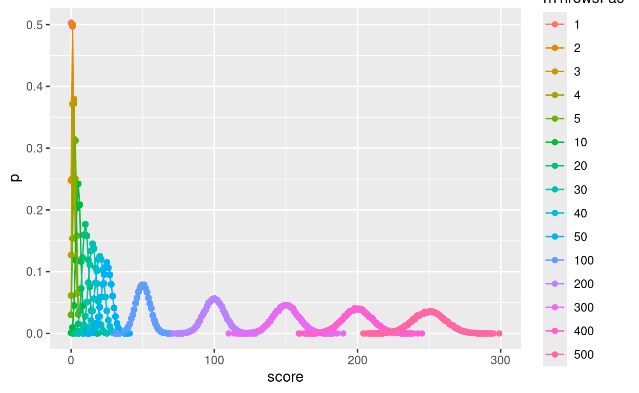
Show code
ggsave(filename = "tossingCoins1.png",
       width = 1700,
       height = 1470,
       units = "px")


ggplot(data = tibBinom,
       aes(x = scaledScore, y = p, colour = nThrowsFac)) +
  geom_point() +
  geom_line()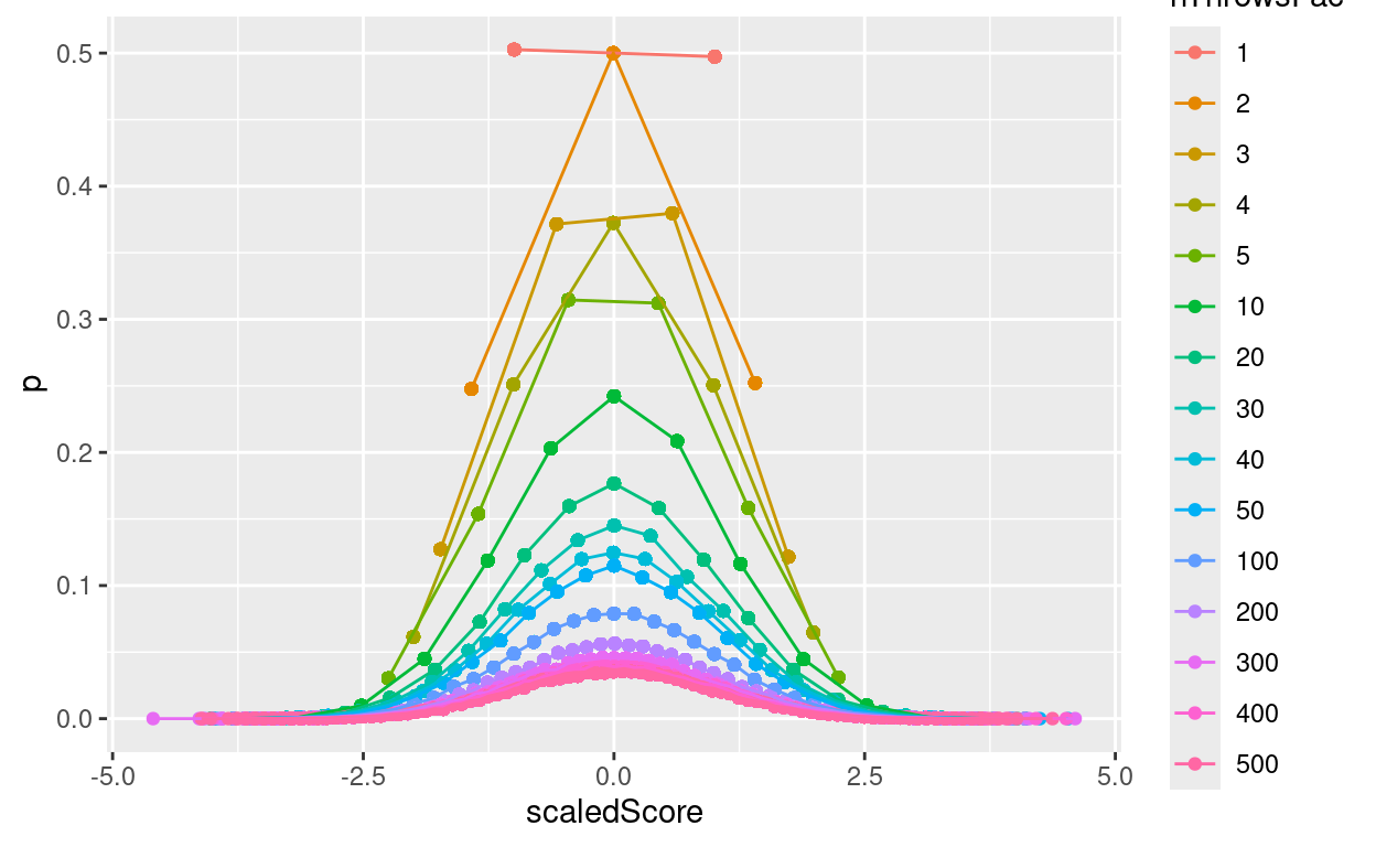
Show code
ggsave(filename = "tossingCoinsScaled.png",
       width = 1700,
       height = 1470,
       units = "px")


pbinom(0:2, 2, .5)
[1] 0.25 0.75 1.00Show code
c(1:5, 10, 20, 50, 100) %>%
  as_tibble() %>%
  rename(nThrows = value) %>%
  rowwise() %>%
  mutate(pVals = list(pbinom(0:nThrows, nThrows, .5))) %>%
  ungroup() %>%
  unnest_longer(pVals) %>%
  group_by(nThrows) %>%
  mutate(score = row_number() - 1,
         nThrowsFac = factor(first(nThrows)),
         p = if_else(row_number() == 1, pVals, pVals - lag(pVals)),
         meanScore = Hmisc::wtd.mean(score, weights = p),
         sdScore = sqrt(Hmisc::wtd.var(score, weights = p, normwt = TRUE)),
         stdScore = (score - meanScore) / sdScore) -> tibpBinom


# tibGauss1 %>%
#   summarise(max(p)) # .399
#
# tibpBinom %>%
#   filter(nThrows == 100) %>%
#   summarise(max(p)) # .0796

ggplot(data = tibpBinom,
       aes(x = stdScore, y = p, colour = nThrowsFac)) +
  geom_point() +
  geom_line() +
  geom_line(inherit.aes = FALSE,
            data = tibGauss1,
            aes(x = value, y = p * .0796 / .399)) +
  ylab("Probability") +
  xlab("Standardised score across tossing n fair coins, heads = 1, tails = 0") +
  scale_colour_discrete(name = "n(throws)")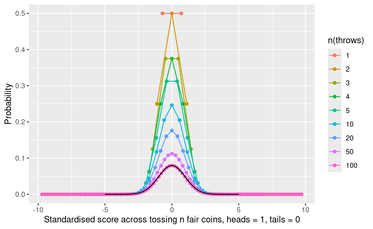
Show code
ggsave(filename = "pbinomWithGauss.png",
       width = 1700,
       height = 1470,
       units = "px")
Variance: Gaussian
Show code
seq(0, 20, length = 5001) %>%
  as_tibble() %>%
  mutate(NHS = dnorm(value, 8, 2),
         HS = dnorm(value, 12, 1)) %>%
  pivot_longer(cols = ends_with("HS"), names_to = "Population", values_to = "p") -> tibGauss2

ggplot(data = tibGauss2,
       aes(x = value, y = p, colour = Population)) +
  geom_line(size = 2, alpha = .8) +
  xlab("Observed score") +
  ylab("Probability")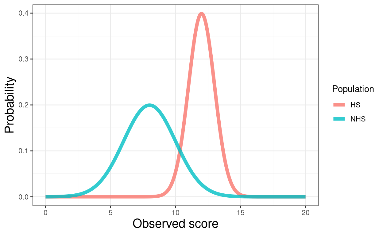
Show code
ggsave(filename = "Gauss2.png",
       width = 1700,
       height = 1470,
       units = "px")
Variance: real, from CORE-OM items
Show code
# tmpDatDir <- "~/internalHDD/Data/CORE/translations/SPA_other/Clara/Our_papers/NClinPaper"
tmpDatDir <- "/media/chris/Clevo_SSD2/Data/CORE/translations/SPA_other/Clara/Our_papers/2020_NClinPaper"
readxl::read_excel(paste0(tmpDatDir, "/", "Muestra_NoClinica_CP180520.xlsx")) %>%
  mutate(Gender = recode(Genero,
                         Masculino = "Male",
                         Femenino = "Female")) -> tibRawDat

### this is a silly way to get around having to up the na.rm = TRUE clause in the mutate
meanNotNA <- function(x){
  mean(x, na.rm = TRUE)
}
medianNotNA <- function(x){
  median(x, na.rm = TRUE)
}
varNotNA <- function(x){
  var(x, na.rm = TRUE)
}
sdNotNA <- function(x){
  sd(x, na.rm = TRUE)
}
minNotNA <- function(x){
  min(x, na.rm = TRUE)
}
maxNotNA <- function(x){
  max(x, na.rm = TRUE)
}

# tibRawDat %>%
#   select(starts_with("COREOM01")) %>%
#   corrr::correlate(diagonal = 1) %>%
#   pivot_longer(cols = -term) %>%
#   filter(term != name) %>%
#   arrange(desc(value))
### OK, all recoded

tibRawDat %>%
  filter(Excluded == "NO" & !is.na(Genero)) -> tibUseDat

tibUseDat %>%
  select(Gender, Edad, starts_with("COREOM01")) %>%
  select(-COREOM01_35) %>%
  pivot_longer(cols = starts_with("COREOM01"), names_to = "Item", values_to = "Score") %>%
  # group_by(Gender, Item) %>%
  group_by(Item) %>%
  summarise(totN = n(),
            nOK = getNOK(Score),
            min = minNotNA(Score),
            mean = meanNotNA(Score),
            median = medianNotNA(Score),
            max = maxNotNA(Score),
            var = varNotNA(Score),
            sd = sdNotNA(Score)) %>%
  ungroup() %>%
  # filter(min != 0 | max != 4) ## OK full range on all items
  arrange(var) %>%
  filter(row_number() %in% c(1,2,3, 32, 33, 34)) -> tmpTibSummary

tmpTibSummary %>%
  select(Item) %>%
  pull() -> tmpVecItems

c("R: plans to end my life",
  "R: hurt myself physically...",
  "R: threatened or intimidated",
  "P: difficulty getting to sleep ...",
  "P: thought to blame ...",
  "P: felt unhappy") -> tmpVecNames

tibUseDat %>%
  select(all_of(tmpVecItems)) -> tmpTibRawScores

tmpTibRawScores %>%
  pivot_longer(cols = everything(), names_to = "Item", values_to = "Score") %>%
  filter(!is.na(Score)) %>%
  mutate(Item = ordered(Item,
                        levels = tmpVecItems,
                        labels = tmpVecNames)) -> tmpTibLongScores

tmpTibSummary %>%
  mutate(Item = ordered(Item,
                        levels = tmpVecItems,
                        labels = tmpVecNames),
         meanMinusSD = mean - sd,
         meanPlusSD = mean + sd) -> tmpTibSummary


ggplot(data = tmpTibLongScores,
       aes(x = Score)) +
  ylim(0, 1000) +
  geom_bar(width = 1) +
  geom_vline(data = tmpTibSummary,
             aes(xintercept = mean),
             colour = "green") +
  facet_wrap(facets = vars(Item), ncol = 3)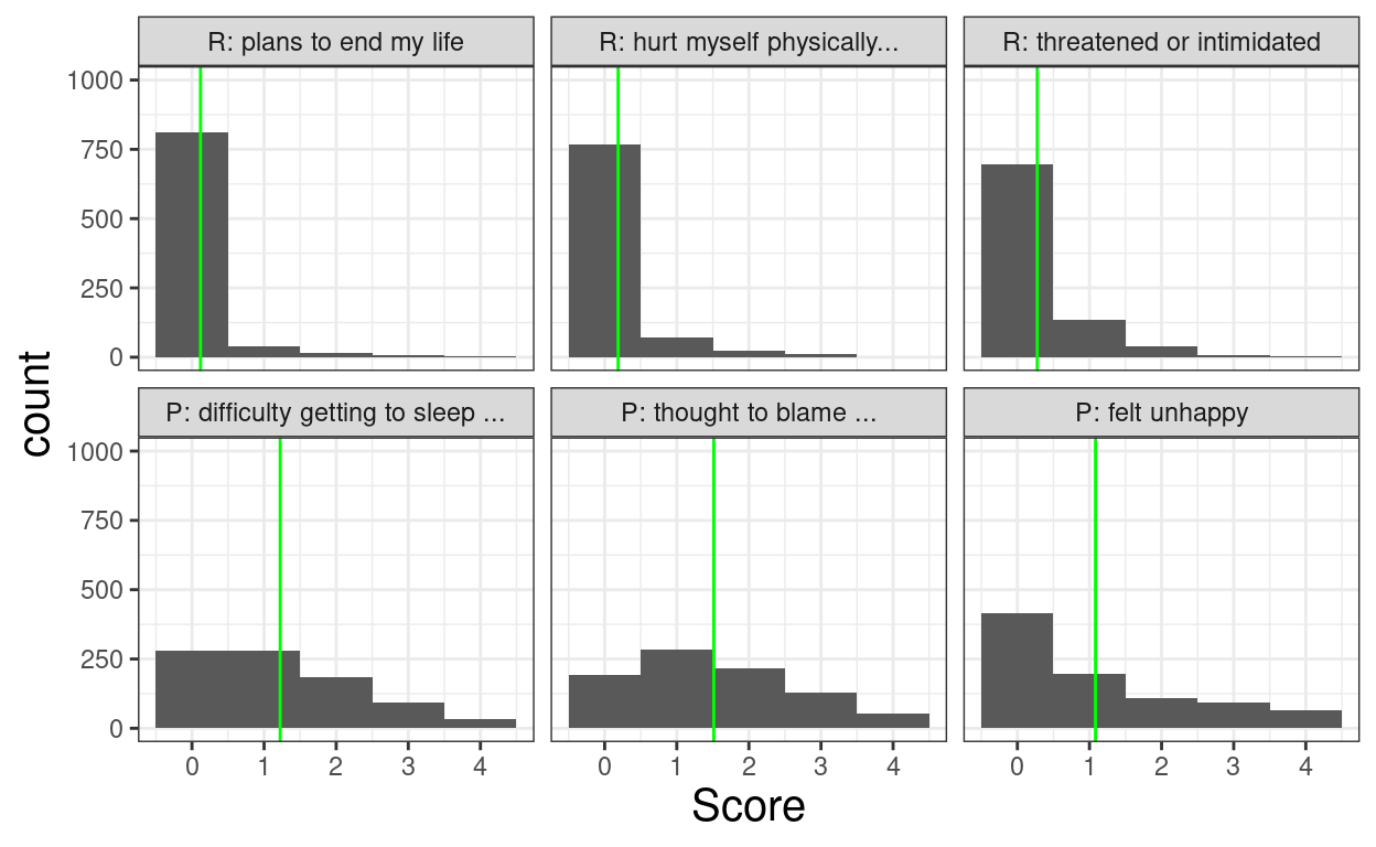
Show code
ggsave(filename = "Variance1.png",
       width = 1700,
       height = 1470,
       units = "px")


ggplot(data = tmpTibLongScores,
       aes(x = Score)) +
  ylim(0, 1000) +
  geom_bar(width = 1) +
  geom_vline(data = tmpTibSummary,
             aes(xintercept = mean),
             colour = "green") +
  geom_segment(inherit.aes = FALSE,
               data = tmpTibSummary,
               aes(y = 900, yend = 900,
                   x = meanMinusSD,
                   xend = meanPlusSD),
               colour = "blue",
               lineend = "round",
               arrow = arrow(ends = "both",
                             length = unit(2, "mm"))) +
  geom_text(data = tmpTibSummary,
            aes(y = 960, x = 4.5, label = paste0("Mean: ",
                                                 round(mean, 2),
                                                 "\nVar: ",
                                                 round(var, 2),
                                                 "\nSD: ",
                                                 round(sd, 2))),
            size = 2.5,
            hjust = 1,
            vjust = 1) +
  facet_wrap(facets = vars(Item), ncol = 3)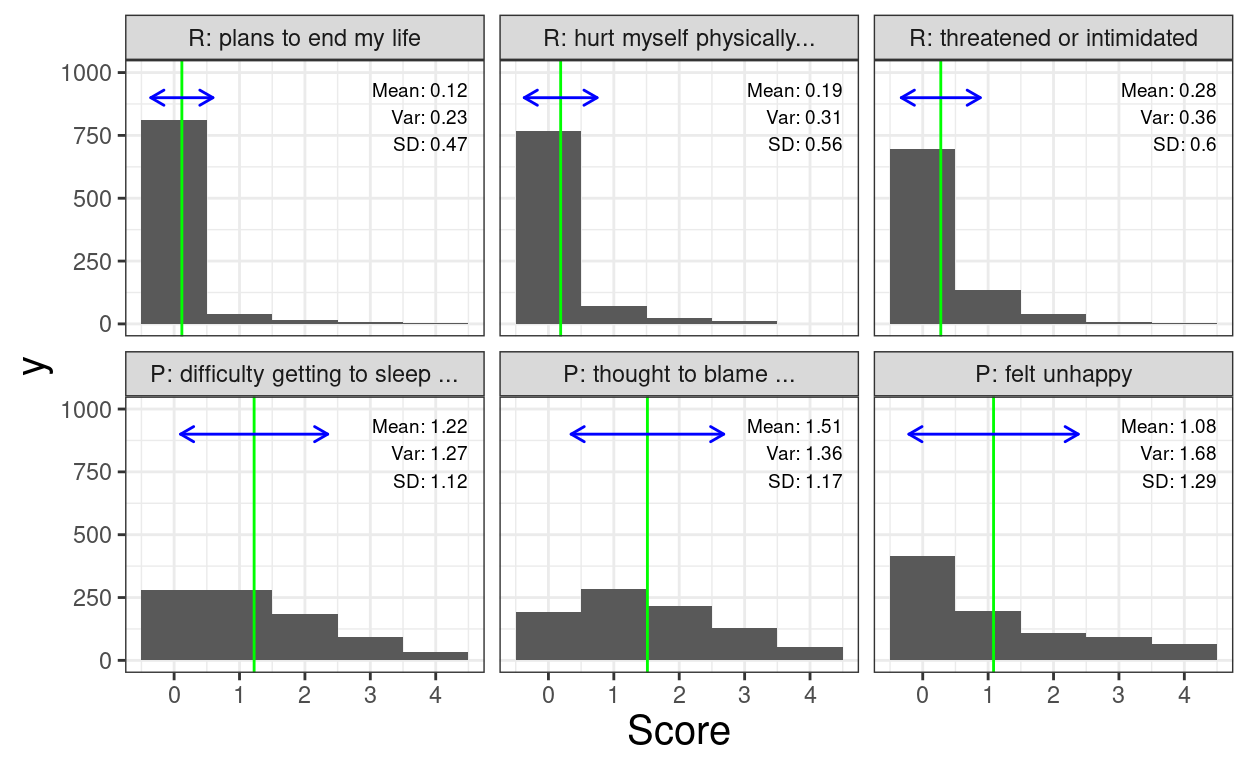
Show code
ggsave(filename = "Variance2.png",
       width = 1700,
       height = 1470,
       units = "px")
Histograms and barplots
Show code
ggplot(data = tibRawDat,
       aes(x = Gender)) +
  geom_bar() +
  xlab("Gender") +
  theme(axis.text = element_text(size = 40),
        axis.title = element_text(size = 50)) -> ggGender1

ggplot(data = tibRawDat,
       aes(x = Edad)) +
  geom_histogram(center = TRUE,
                 breaks = 18:80) +
  xlab("Age") +
  theme(axis.text = element_text(size = 40),
        axis.title = element_text(size = 50)) -> ggAge1

ggpubr::ggarrange(ggGender1, ggAge1) -> ggArrange1

ggpubr::ggexport(ggArrange1,
         filename = "Histogram1.png",
         width = 1700,
         height = 1470,
         units = "px")
[1] "Histogram1%03d.png"Show code
ggplot(data = tibRawDat,
       aes(x = Edad)) +
  geom_histogram(center = TRUE,
                 breaks = c(18, 20, 30, 40, 50, 80),
                 closed = "right") +
  xlab("Age") +
  scale_x_continuous(breaks = seq(10, 80, 10))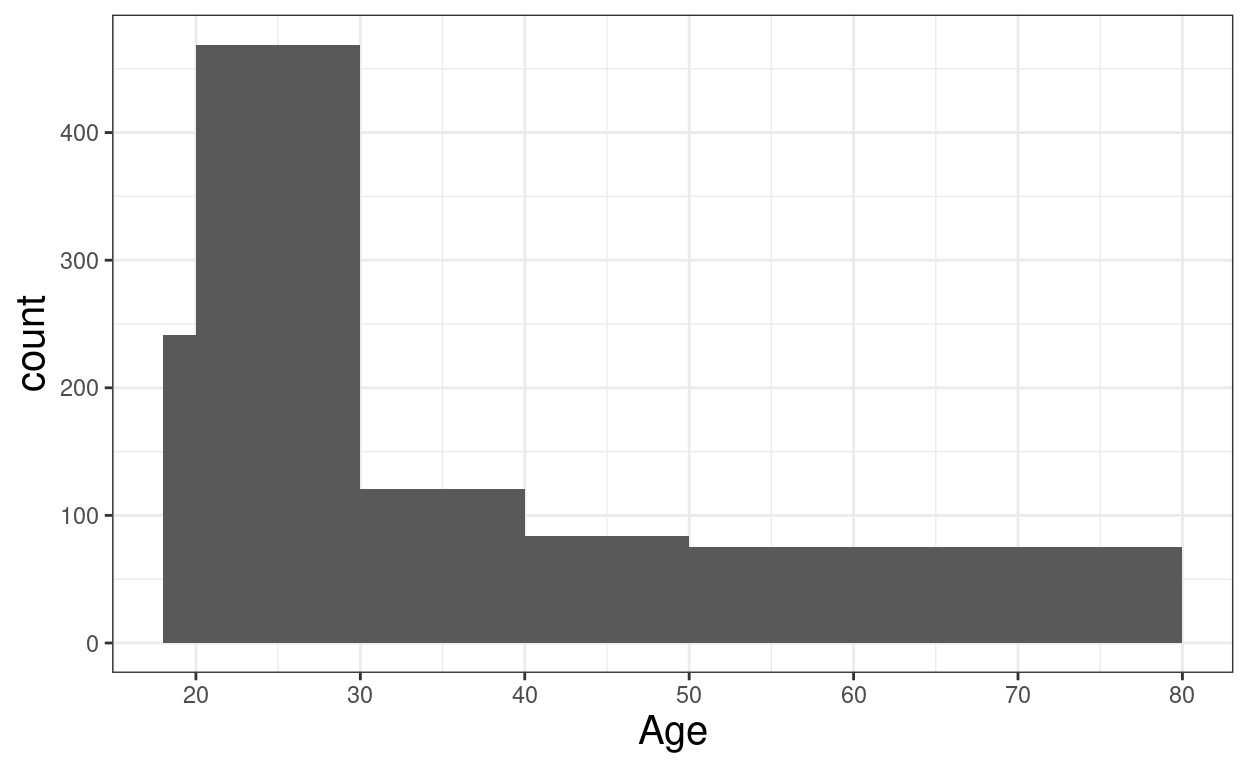
Show code
  # theme(axis.text = element_text(size = 40),
  #       axis.title = element_text(size = 50))

ggsave(filename = "HistAge.png",
       width = 1700,
       height = 1470,
       units = "px")

ggplot(data = tibRawDat,
       aes(x = Edad)) +
  geom_histogram(aes(y = stat(count) / sum(count)),
                 center = TRUE,
                 breaks = c(18, 20, 30, 40, 50, 80),
                 closed = "right") +
  xlab("Age") +
  ylab("Proportion") +
  scale_x_continuous(breaks = seq(10, 80, 10))
Show code
  # theme(axis.text = element_text(size = 40),
  #       axis.title = element_text(size = 50))

ggsave(filename = "HistAge2.png",
       width = 1700,
       height = 1470,
       units = "px")

ggplot(data = tibRawDat,
       aes(x = Edad, fill = Gender)) +
  geom_histogram(aes(y = stat(count) / sum(count)),
                 position = "dodge2",
                 center = TRUE,
                 breaks = c(18, seq(20, 80, 10)),
                 closed = "left") +
  xlab("Age") +
  ylab("Proportion") +
  scale_x_continuous(breaks = seq(20, 80, 5))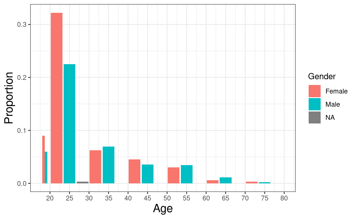
Show code
ggsave(filename = "HistAgeGendDodge.png",
       width = 1700,
       height = 1470,
       units = "px")


ggplot(data = tibRawDat,
       aes(x = Edad, fill = Gender)) +
  geom_histogram(aes(y = stat(count) / sum(count)),
                 position = "stack",
                 center = TRUE,
                 breaks = c(18, seq(20, 80, 10)),
                 closed = "left") +
  xlab("Age") +
  ylab("Proportion") +
  scale_x_continuous(breaks = seq(20, 80, 5))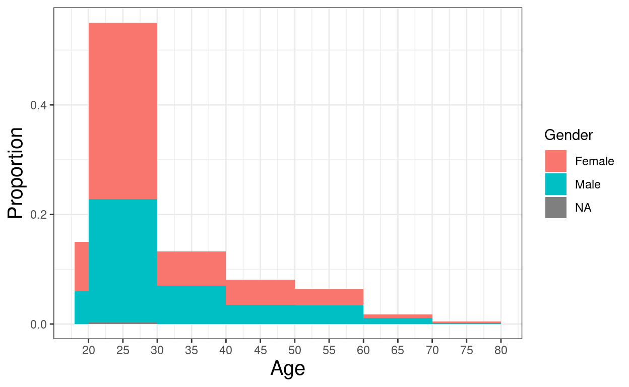
Show code
ggsave(filename = "HistAgeGendStack.png",
       width = 1700,
       height = 1470,
       units = "px")


tibRawDat %>%
  filter(!is.na(Edad)) %>%
  mutate(Age = case_when(Edad < 20 ~ "<20",
                         Edad < 30 ~ "20 to 29",
                         Edad < 40 ~ "30 to 39",
                         Edad < 50 ~ "40 to 49",
                         Edad >= 50 ~ "50 and over"),
         Age = ordered(Age,
                       levels = c("<20",
                                  "20 to 29",
                                  "30 to 39",
                                  "40 to 49",
                                  "50 and over"))) -> tmpTib #%>% select(Edad, Age)

tmpTib %>%
  tabyl(Age) %>%
  adorn_pct_formatting(digits = 1) %>%
pander(justify = "lrr")| Age | n | percent |
|---|---|---|
| <20 | 148 | 14.9% |
| 20 to 29 | 545 | 55.1% |
| 30 to 39 | 131 | 13.2% |
| 40 to 49 | 80 | 8.1% |
| 50 and over | 86 | 8.7% |
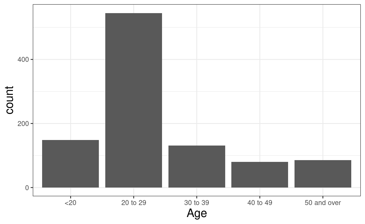
Show code
ggsave(filename = "BarAge.png",
       width = 1700,
       height = 1470,
       units = "px")
Boxplots: Gaussian
Show code
# A tibble: 1 × 5
    min   lwrQ   median  uprQ   max
  <dbl>  <dbl>    <dbl> <dbl> <dbl>
1 -3.88 -0.664 0.000494 0.663  3.36
Show code
ggplot(data = tmpTibGaussian,
       aes(y = value)) +
  geom_boxplot(fill = "grey") +
  ylim(4, 4) +
  xlab("") -> ggGaussBox1

ggGaussBox1
Show code
ggsave(filename = "GaussBox1.png",
       width = 1700,
       height = 1470,
       units = "px")

ggplot(data = tmpTibGaussian,
       aes(y = value)) +
  geom_boxplot(fill = "grey") +
  ylim(-4, 4) +
  xlab("") +
  theme(axis.text = element_text(size = 40),
        axis.title = element_text(size = 50)) -> ggGaussBox2

ggGaussBox2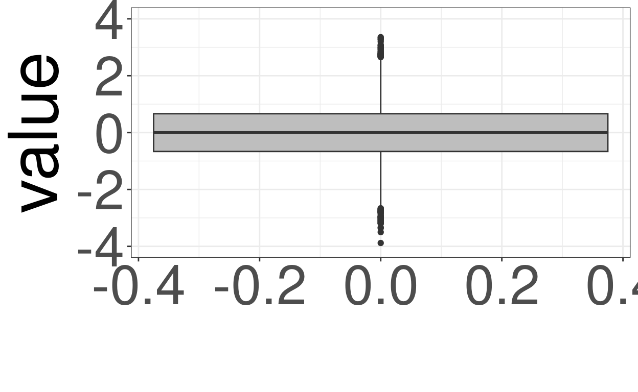
Show code
ggplot(data = tmpTibGaussian,
       aes(x = value)) +
  geom_histogram(aes(y = ..density..),
                 fill = "grey") +
  geom_vline(xintercept = median(tmpTibGaussian$value)) +
  geom_line(data = tibGauss1,
            aes(x = value, y = p)) +
  ylab("Probability") -> ggGaussHistOnX

ggGaussHistOnX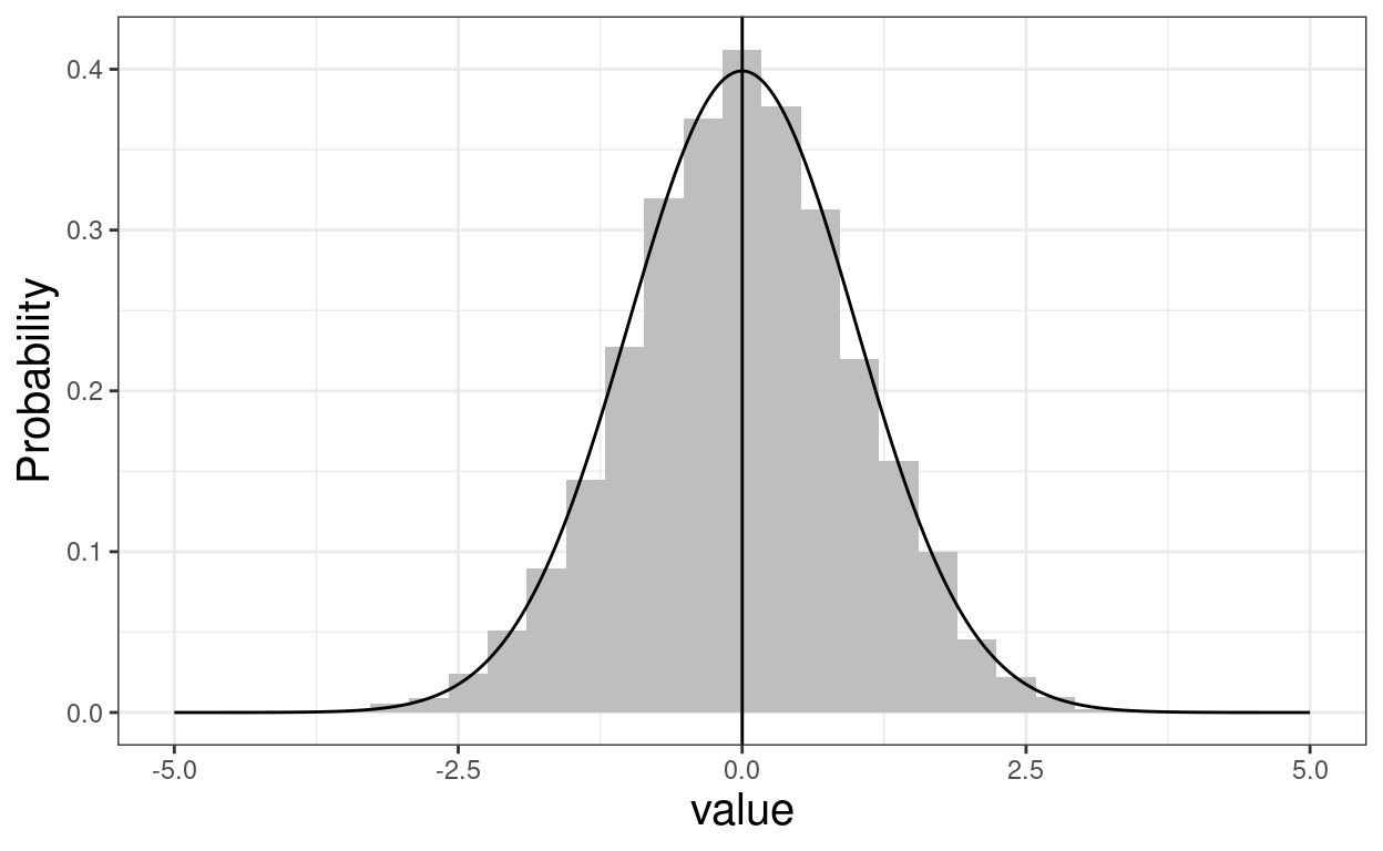
Show code
ggsave(filename = "GaussHistOnX.png",
       width = 1700,
       height = 1470,
       units = "px")

ggplot(data = tmpTibGaussian,
       aes(y = value)) +
  geom_histogram(aes(x = ..density..),
                 fill = "grey") +
  geom_hline(yintercept = median(tmpTibGaussian$value)) +
  geom_line(data = tibGauss1,
            aes(y = value, x = p),
            orientation = "y") +
  ylim(-4, 4) +
  xlab("") +
  ylab("") +
  theme(axis.text = element_text(size = 40),
        axis.title = element_text(size = 50)) -> ggGaussHistOnY

ggGaussHistOnY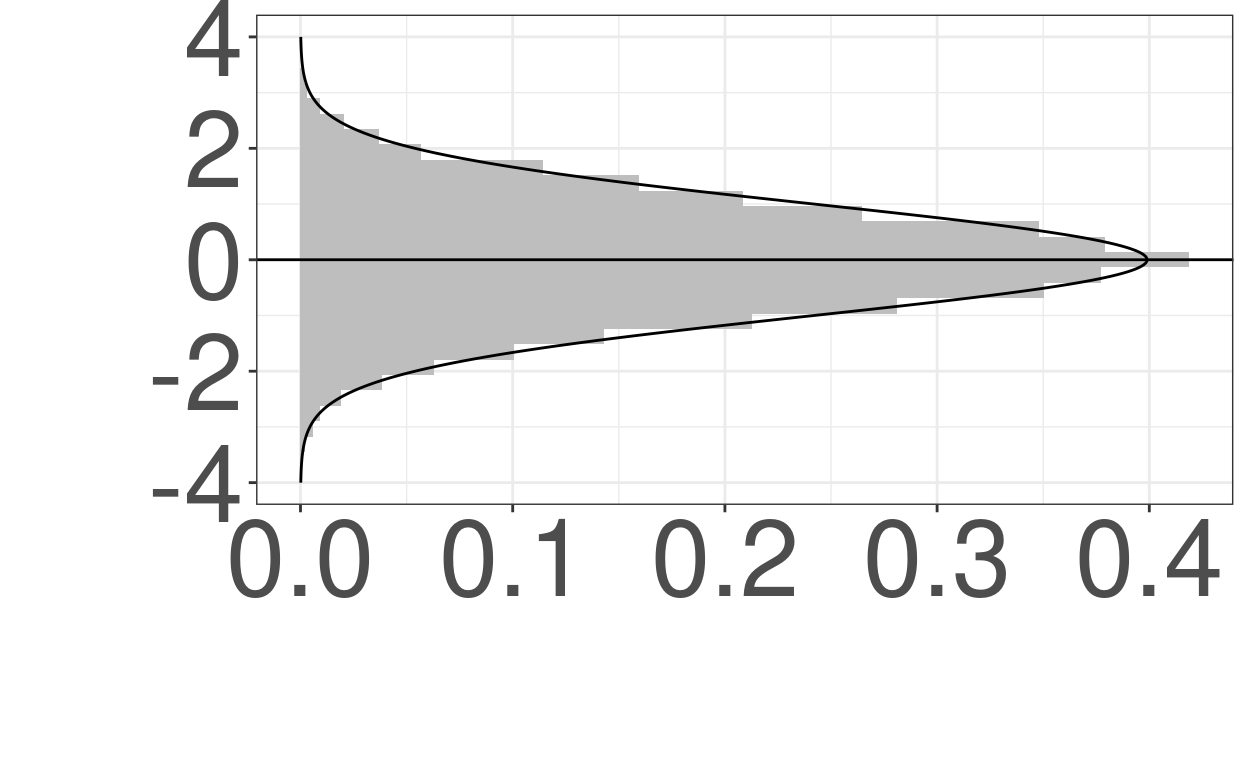
Show code
ggpubr::ggarrange(ggGaussBox2, ggGaussHistOnY,
                  ncol = 2) -> ggArrange2

ggArrange2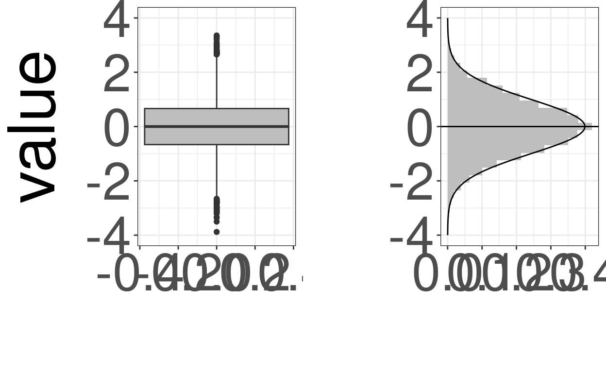
Show code
ggpubr::ggexport(ggArrange2,
         filename = "BoxAndHist.png",
         width = 1700,
         height = 1470,
         units = "px")
[1] "BoxAndHist%03d.png"Boxplots: real, age and CORE-OM scores
Show code
ggplot(data = tibRawDat,
       aes(y = Edad, x = Gender, fill = Gender)) +
  geom_boxplot(varwidth = TRUE) +
  ylab("Age")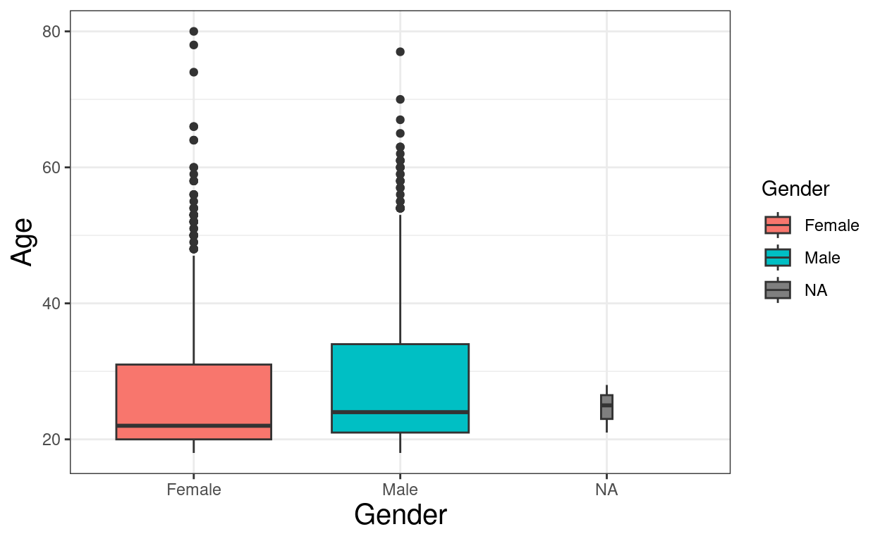
Show code
ggsave(filename = "AgeByGenderBox.png",
       width = 1700,
       height = 1470,
       units = "px")

tibRawDat %>%
  mutate(SocState = `Estado civil`,
         SocState = recode(SocState,
                           `Casado/a` = "Coupled",
                           `Soltero`  = "Single",
                           `Separado/a` = "Separated",
                           `Divorciado/a` = "Divorced",
                           `Unido/a` = "Coupled",
                           `Unido` = "Coupled",
                           `Viudo/a` = "Widowed/Widower")) %>%
  rowwise() %>%
  mutate(meanCOREOM = meanNotNA(c_across(COREOM01_01:COREOM01_34))) %>%
  ungroup() -> tibRawDat

tibRawDat %>%
  mutate(SocStatNA = if_else(is.na(SocState), "NA", SocState)) %>%
  group_by(SocStatNA) %>%
  summarise(tmpN = n(),
            tmpMedianAge = median(Edad, na.rm = TRUE),
            varAge = var(Edad, na.rm = TRUE),
            SDAge = sqrt(varAge)) -> tmpTib

tmpTib %>%
  arrange(desc(tmpN)) %>%
  select(SocStatNA) %>%
  pull() -> tmpVecN

tmpTib %>%
  arrange(tmpMedianAge) %>%
  select(SocStatNA) %>%
  pull() -> tmpVecAge


tibRawDat %>%
  mutate(SocStatNA = if_else(is.na(SocState), "NA", SocState),
         SocStatN = ordered(SocStatNA,
                            levels = tmpVecN,
                            labels = tmpVecN),
         SocStateAge = ordered(SocStatNA,
                               levels = tmpVecAge,
                               labels = tmpVecAge)) -> tibRawDat

ggplot(data = tibRawDat,
       aes(y = Edad, x = SocStatN, fill = SocStatN)) +
  geom_boxplot(varwidth = TRUE) +
  geom_text(data = tmpTib,
            inherit.aes = FALSE,
            aes(x = SocStatNA, y = 12, label = tmpN),
            vjust = .5) +
  geom_text(x = .5, y = 12, label = "n: ",
            vjust = .5,
            hjust = 0) +
  ylim(10, 80) +
  scale_fill_discrete(name = "Social status") +
  ylab("Age") +
  xlab("Social status") +
  theme(axis.text.x = element_text(angle = 70, hjust = 1))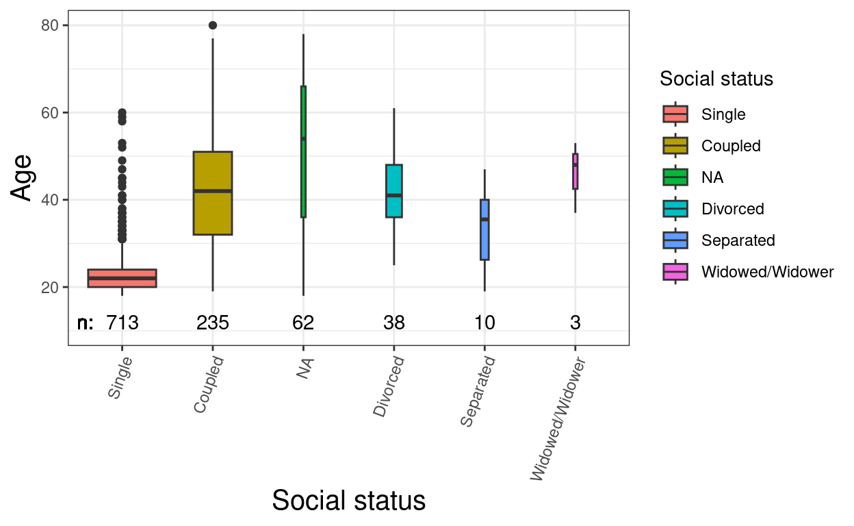
Show code
ggsave(filename = "AgeBySocStatnBox.png",
       width = 1700,
       height = 1470,
       units = "px")

ggplot(data = tibRawDat,
       aes(y = meanCOREOM, x = SocStatN, fill = SocStatN)) +
  geom_boxplot(varwidth = TRUE) +
  geom_text(data = tmpTib,
            inherit.aes = FALSE,
            aes(x = SocStatNA, y = -.2, label = tmpN),
            vjust = .5) +
  geom_text(x = .5, y = -.2, label = "n: ",
            vjust = .5,
            hjust = 0) +
  ylim(-.5, 4) +
  scale_fill_discrete(name = "Social status") +
  ylab("CORE-OM score (mean item score)") +
  xlab("Social status") +
  theme(axis.text.x = element_text(angle = 70, hjust = 1))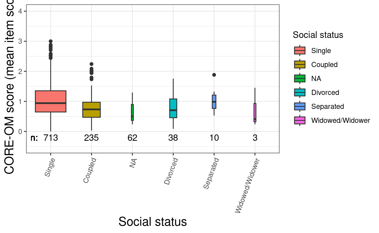
Show code
ggsave(filename = "COREOMBySocStatnBox.png",
       width = 1700,
       height = 1470,
       units = "px")

tibRawDat %>%
  filter(!is.na(`Tiene Hijos`)) %>%
  mutate(nChildren = `Especifique cuántos`,
         nChildren = if_else(nChildren > 3, 4, nChildren),
         nChildren = if_else(`Tiene Hijos` == "NO", 0, nChildren),
         nChildren = ordered(nChildren,
                             levels = 0:4,
                             labels = c(as.character(0:3),
                                        "4 or more"))) %>%
  filter(!is.na(nChildren)) -> tmpTib

ggplot(data = tmpTib,
       aes(y = Edad, x = nChildren, fill = nChildren)) +
geom_boxplot(varwidth = TRUE) 
Show code

Notched boxplots: Gaussian
Show code
tmpTibGaussian %>%
  filter(row_number() <= 500) %>%
  mutate(samp250 = if_else(row_number() <= 250, value, NA_real_),
         samp100 = if_else(row_number() <= 100, value, NA_real_),
         samp50 = if_else(row_number() <= 50, value, NA_real_),
         samp10 = if_else(row_number() <= 10, value, NA_real_)) %>%
  rename(samp500 = value) -> tmpTib

tmpTib %>%
  pivot_longer(cols = everything(), names_to = "sample") %>%
  mutate(sample = ordered(sample,
                          levels = paste0("samp", c(500, 250, 100, 50, 10)))) -> tmpTibLong

ggplot(data = tmpTib,
       aes(y = samp250)) +
  geom_boxplot(fill = "grey", varwidth = TRUE, notch = TRUE) +
  ylim(-4, 4) +
  xlab("") +
  ylab("value") +
  theme(axis.ticks.x = element_blank(),
axis.text.x = element_blank()) 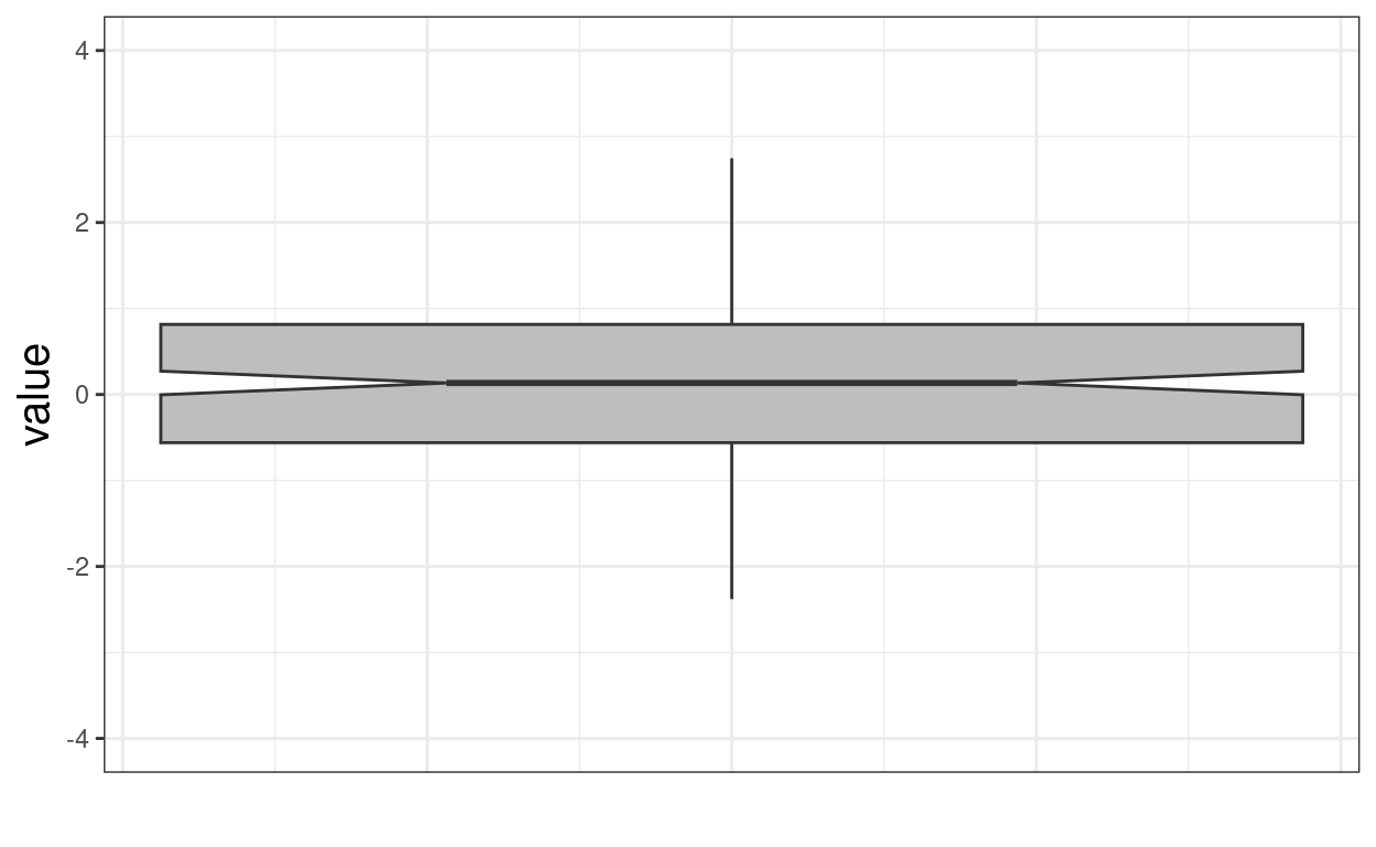
Show code
ggsave(filename = "notchedGaussianBox1.png",
       width = 1700,
       height = 1470,
       units = "px")

ggplot(data = tmpTib,
       aes(y = samp250)) +
  geom_boxplot(fill = "grey", varwidth = TRUE) +
  ylim(-4, 4) +
  xlab("") +
  ylab("value") +
  theme(axis.ticks.x = element_blank(),
axis.text.x = element_blank()) 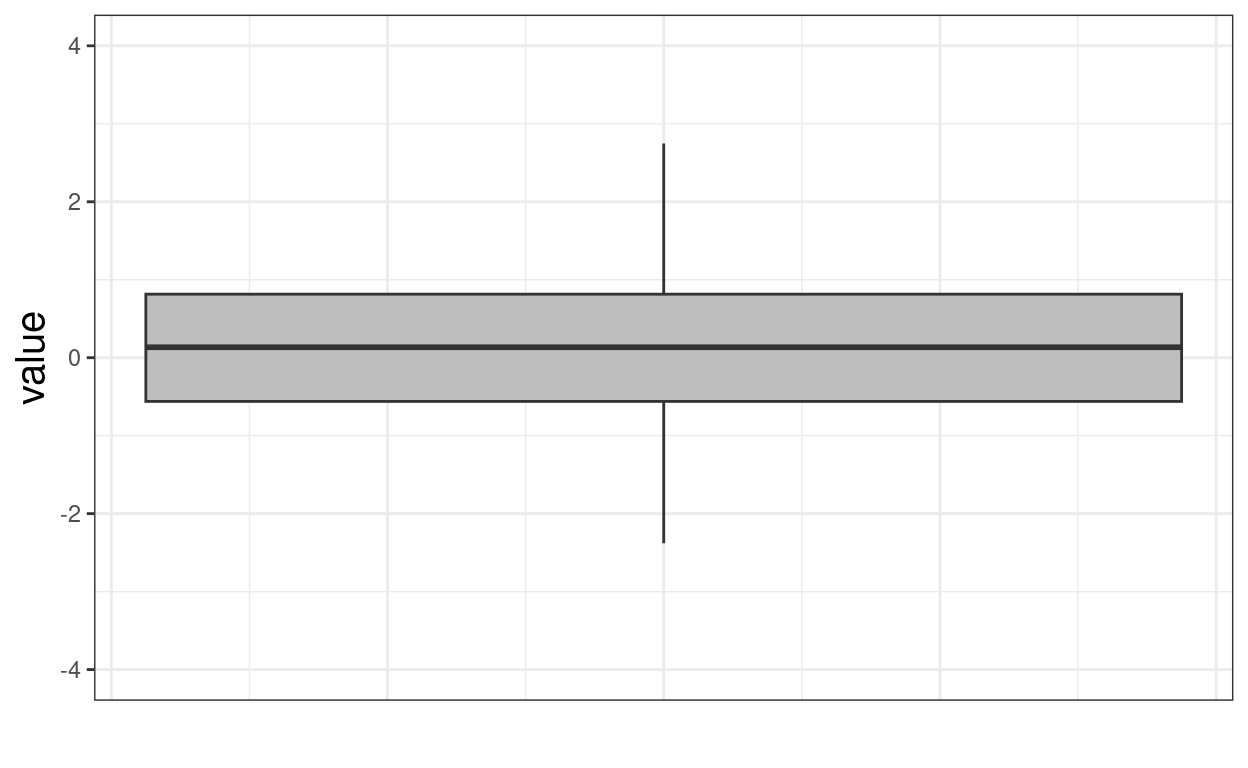
Show code
ggsave(filename = "notNotchedGaussianBox1.png",
       width = 1700,
       height = 1470,
       units = "px")

ggplot(data = tmpTibLong,
       aes(y = value)) +
  geom_boxplot(fill = "grey", varwidth = TRUE, notch = TRUE) +
  geom_hline(yintercept = 0) +
  ylim(-4, 4) +
  facet_grid(cols = vars(sample)) +
  xlab("") +
  theme(axis.ticks.x = element_blank(),
axis.text.x = element_blank()) 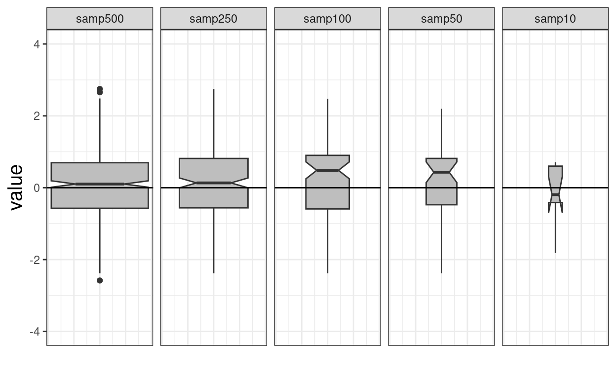
Show code
ggsave(filename = "notchedGaussianBoxes2.png",
       width = 1700,
       height = 1470,
       units = "px")

tmpTibGaussian %>%
  mutate(simulN = row_number() %% 20) %>%
  group_by(simulN) %>%
  mutate(samp250 = if_else(row_number() <= 250, value, NA_real_),
         samp100 = if_else(row_number() <= 100, value, NA_real_),
         samp50 = if_else(row_number() <= 50, value, NA_real_),
         samp10 = if_else(row_number() <= 10, value, NA_real_)) %>%
  rename(samp500 = value) %>%
  ungroup() -> tmpTib

tmpTib %>%
  filter(simulN > 1 & simulN <= 5) %>%
  pivot_longer(cols = -simulN, names_to = "sample") %>%
  mutate(sample = ordered(sample,
                          levels = paste0("samp", c(500, 250, 100, 50, 10)))) -> tmpTibLong

ggplot(data = tmpTibLong,
       aes(y = value)) +
  geom_boxplot(fill = "grey", varwidth = TRUE, notch = TRUE) +
  geom_hline(yintercept = 0) +
  ylim(-4, 4) +
  facet_grid(cols = vars(sample),
             rows = vars(simulN)) +
  xlab("") +
  theme(axis.ticks.x = element_blank(),
axis.text.x = element_blank()) 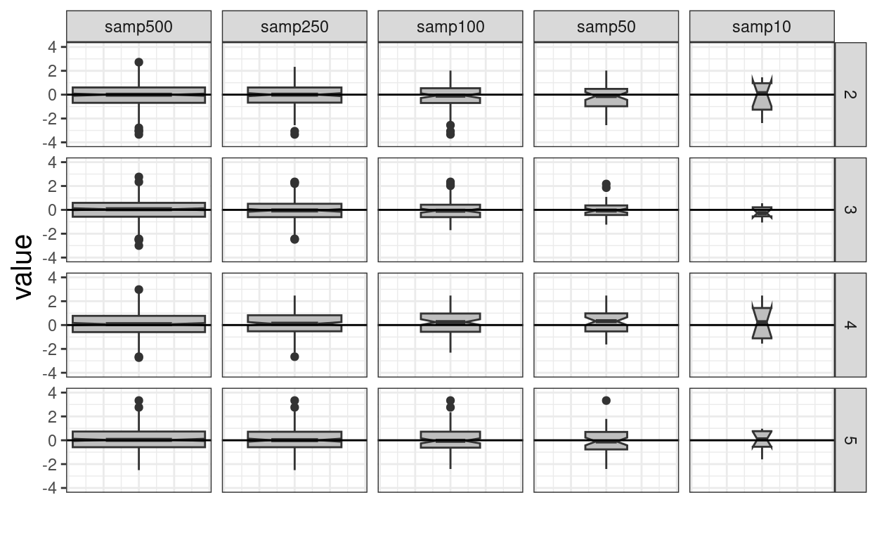
Show code
ggsave(filename = "notchedGaussianBoxes3.png",
       width = 1700,
       height = 1470,
       units = "px")
Notched boxplots: real, age & CORE-OM scores
Show code
tibRawDat %>%
  group_by(Gender) %>%
  summarise(n = n(),
            median = median(Edad, na.rm = TRUE)) -> tmpTibSummary

ggplot(data = tibRawDat,
       aes(y = Edad, x = Gender, fill = Gender)) +
  geom_boxplot(varwidth = TRUE, notch = TRUE) +
  geom_text(data = tmpTibSummary,
            aes(x = Gender, y = 14, label = n),
            vjust = 0) +
  geom_text(x = .90, y = 14, label = "n: ",
            hjust = 1,
            vjust = 0) +
  geom_text(data = tmpTibSummary,
            aes(x = Gender, y = 11, label = median),
            vjust = 0,
            fontface = "plain") +
  geom_text(x = .9, y = 11, label = "median: ",
            hjust = 1,
            vjust = 0,
            fontface = "plain") +
  geom_hline(yintercept = median(tibRawDat$Edad, na.rm = TRUE)) +
  ylab("Age")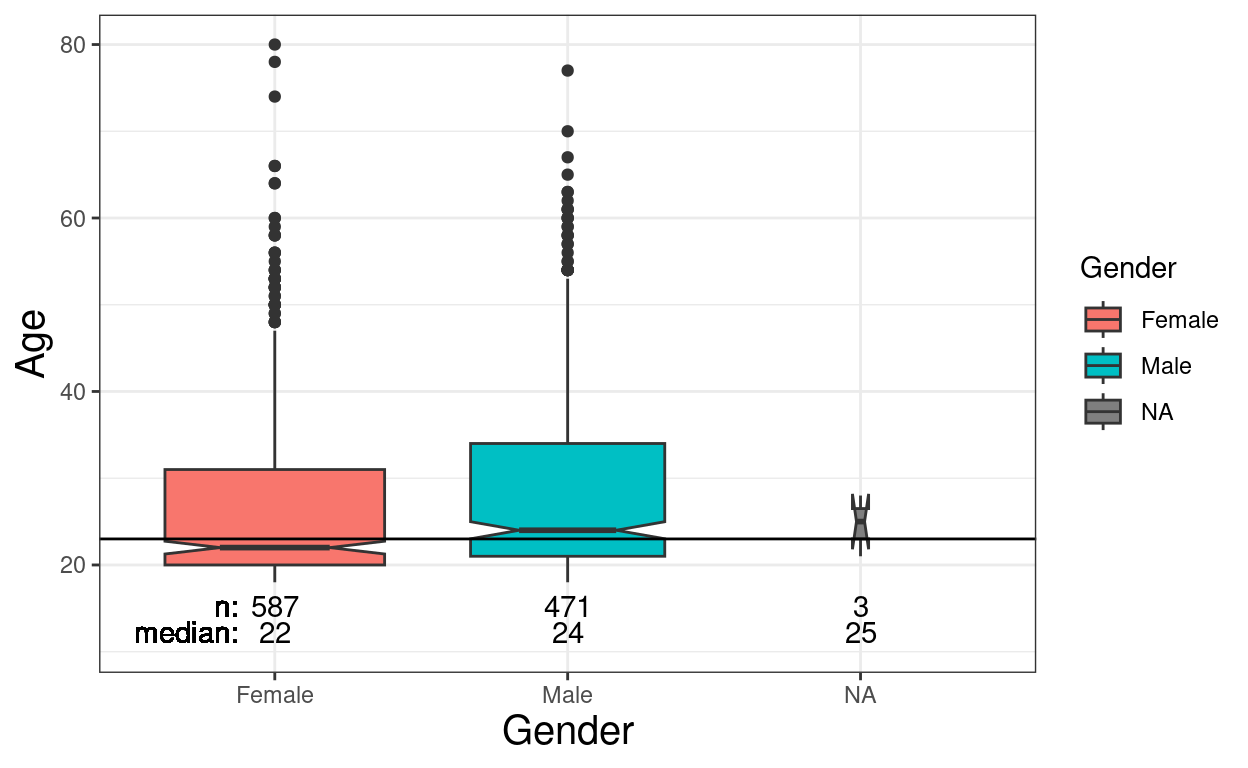
Show code
ggsave(filename = "AgeByGenderNotchedBox.png",
       width = 1700,
       height = 1470,
       units = "px")

tibRawDat %>%
  mutate(SocStatNA = if_else(is.na(SocState), "NA", SocState)) %>%
  group_by(SocStatNA) %>%
  summarise(tmpN = n(),
            tmpMedianAge = median(Edad, na.rm = TRUE),
            varAge = var(Edad, na.rm = TRUE),
            SDAge = sqrt(varAge)) -> tmpTib

tmpTib %>%
  arrange(desc(tmpN)) %>%
  select(SocStatNA) %>%
  pull() -> tmpVecN

tmpTib %>%
  arrange(tmpMedianAge) %>%
  select(SocStatNA) %>%
  pull() -> tmpVecAge


tibRawDat %>%
  mutate(SocStatNA = if_else(is.na(SocState), "NA", SocState),
         SocStatN = ordered(SocStatNA,
                            levels = tmpVecN,
                            labels = tmpVecN),
         SocStateAge = ordered(SocStatNA,
                               levels = tmpVecAge,
                               labels = tmpVecAge)) -> tibRawDat

ggplot(data = tibRawDat,
       aes(y = Edad, x = SocStatN, fill = SocStatN)) +
  geom_boxplot(varwidth = TRUE, notch = TRUE) +
  geom_hline(yintercept = median(tibRawDat$Edad, na.rm = TRUE)) +
  geom_text(data = tmpTib,
            inherit.aes = FALSE,
            aes(x = SocStatNA, y = 12, label = tmpN),
            vjust = .5) +
  geom_text(x = .5, y = 12, label = "n: ",
            vjust = .5,
            hjust = 0) +
  ylim(10, 80) +
  scale_fill_discrete(name = "Social status") +
  ylab("Age") +
  xlab("Social status") +
  theme(axis.text.x = element_text(angle = 70, hjust = 1))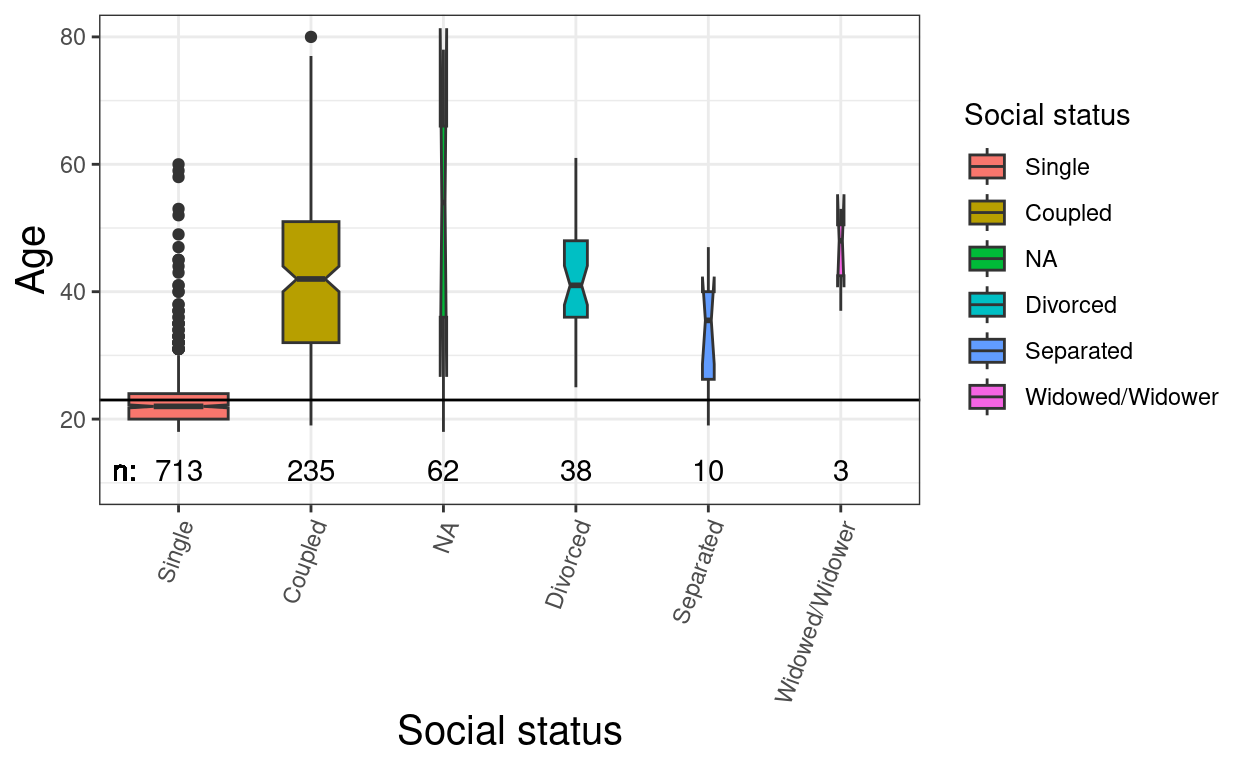
Show code
ggsave(filename = "AgeBySocStatnNotchedBox.png",
width = 1700,
height = 1470,
units = "px")
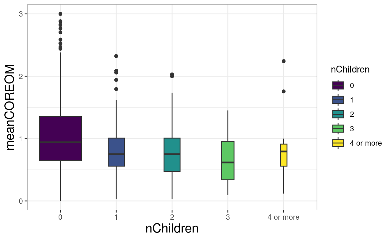
tibRawDat %>%
filter(!is.na(meanCOREOM)) %>%
group_by(SocStatN) %>%
summarise(n = n(),
median = round(median(meanCOREOM), 1)) -> tmpTibSummary
ggplot(data = tibRawDat,
aes(y = meanCOREOM, x = SocStatN, fill = SocStatN)) +
geom_boxplot(varwidth = TRUE, notch = TRUE) +
geom_hline(yintercept = median(tibRawDat$meanCOREOM, na.rm = TRUE)) +
geom_text(data = tmpTibSummary,
inherit.aes = FALSE,
aes(x = SocStatN, y = -.3, label = n),
vjust = .5) +
geom_text(x = .7, y = -.3, label = "n: ",
vjust = .5,
hjust = 1) +
geom_text(data = tmpTibSummary,
inherit.aes = FALSE,
aes(x = SocStatN, y = -.5, label = median),
vjust = .5) +
geom_text(x = .7, y = -.5, label = "median: ",
vjust = .5,
hjust = 1) +
ylim(-.5, 4) +
expand_limits(x = -.7) +
scale_fill_discrete(name = "Social status") +
ylab("CORE-OM score (mean item score)") +
xlab("Social status") +
theme(axis.text.x = element_text(angle = 70, hjust = 1))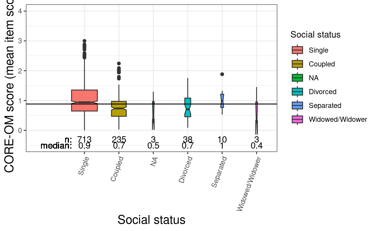
Show code
ggsave(filename = "COREOMBySocStatnBox.png",
       width = 1700,
       height = 1470,
       units = "px")

tibRawDat %>%
  filter(!is.na(`Tiene Hijos`)) %>%
  mutate(nChildren = `Especifique cuántos`,
         nChildren = if_else(nChildren > 3, 4, nChildren),
         nChildren = if_else(`Tiene Hijos` == "NO", 0, nChildren),
         nChildren = ordered(nChildren,
                             levels = 0:4,
                             labels = c(as.character(0:3),
                                        "4 or more"))) %>%
  filter(!is.na(nChildren)) -> tmpTib

ggplot(data = tmpTib,
       aes(y = Edad, x = nChildren, fill = nChildren)) +
geom_boxplot(varwidth = TRUE) 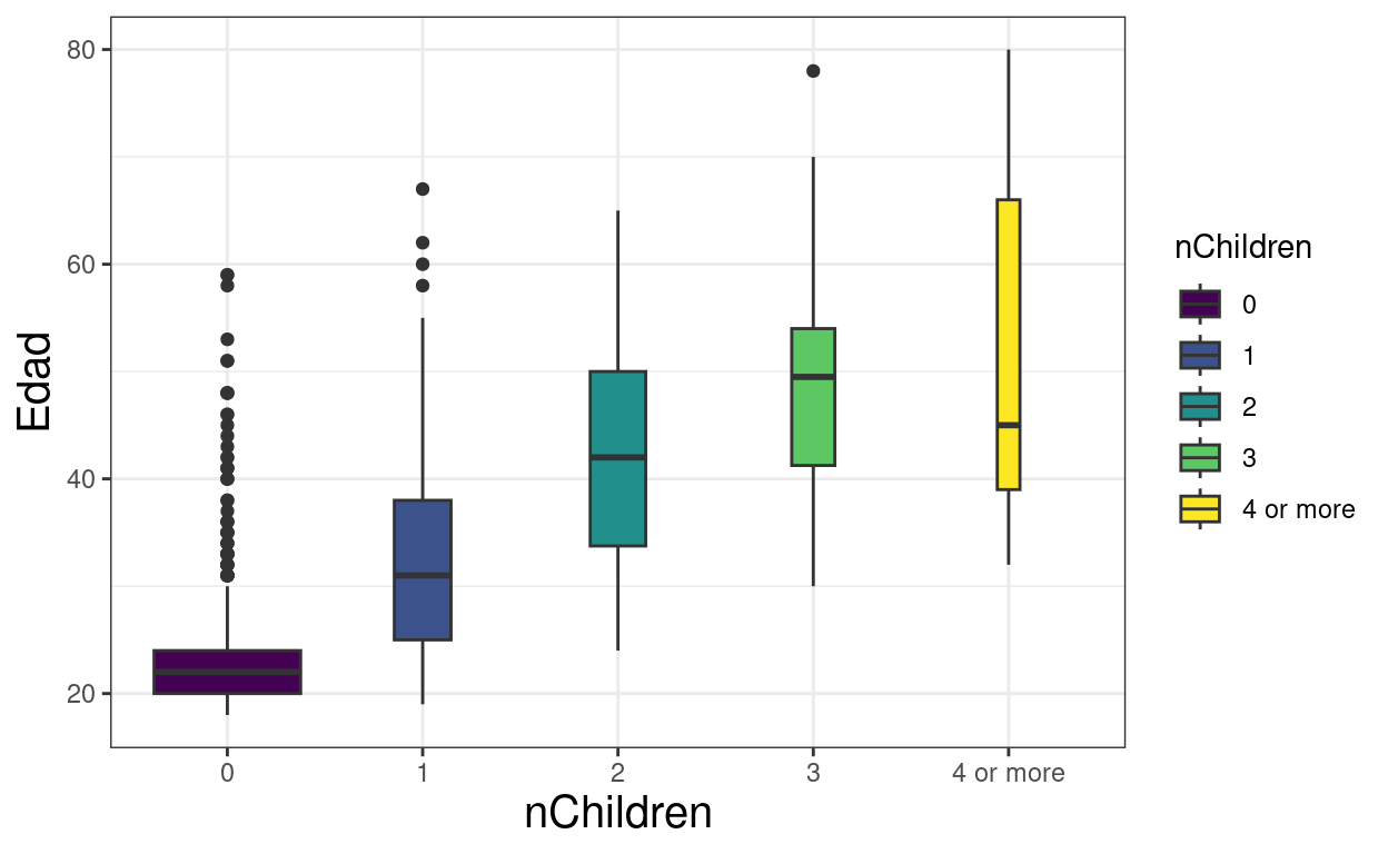
Show code
Violin plot
Show code
### start with simple Gaussian n = 50
set.seed(12345)
tmpValSampN <- 50
1:5 %>%
  as_tibble() %>%
  rename(simN = value) %>%
  group_by(simN) %>%
  mutate(values = list(rnorm(tmpValSampN))) %>%
  ungroup() %>%
  unnest_longer(values) %>%
  mutate(simN = ordered(simN)) -> tmpTib

ggplot(data = filter(tmpTib, simN == 1),
       aes(x = simN, y = values)) +
  geom_violin(fill = "grey") +
  xlab("")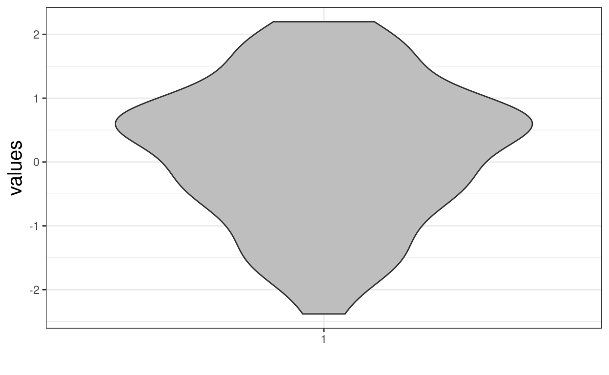
Show code
ggsave(filename = "geomViolin1.png",
       width = 1700,
       height = 1470,
       units = "px")

### add jittered points to the plot
ggplot(data = filter(tmpTib, simN == 1),
       aes(x = simN, y = values)) +
  geom_violin(fill = "grey") +
  geom_jitter(height = 0, width = .07, alpha = .7) +
  xlab("")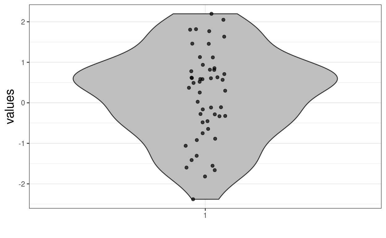
Show code
ggsave(filename = "geomViolin2.png",
       width = 1700,
       height = 1470,
       units = "px")

### no jittering, just transparency
ggplot(data = filter(tmpTib, simN == 1),
       aes(x = simN, y = values)) +
  geom_violin(fill = "grey") +
  geom_point(alpha = .3) +
  xlab("")
Show code
ggsave(filename = "geomViolin3.png",
       width = 1700,
       height = 1470,
       units = "px")


### now use all five simulations
ggplot(data = tmpTib,
       aes(x = simN, y = values)) +
  geom_violin(fill = "grey") +
  geom_jitter(height = 0, width = .07, alpha = .7) +
  geom_hline(yintercept = 0) +
  xlab("Simulations")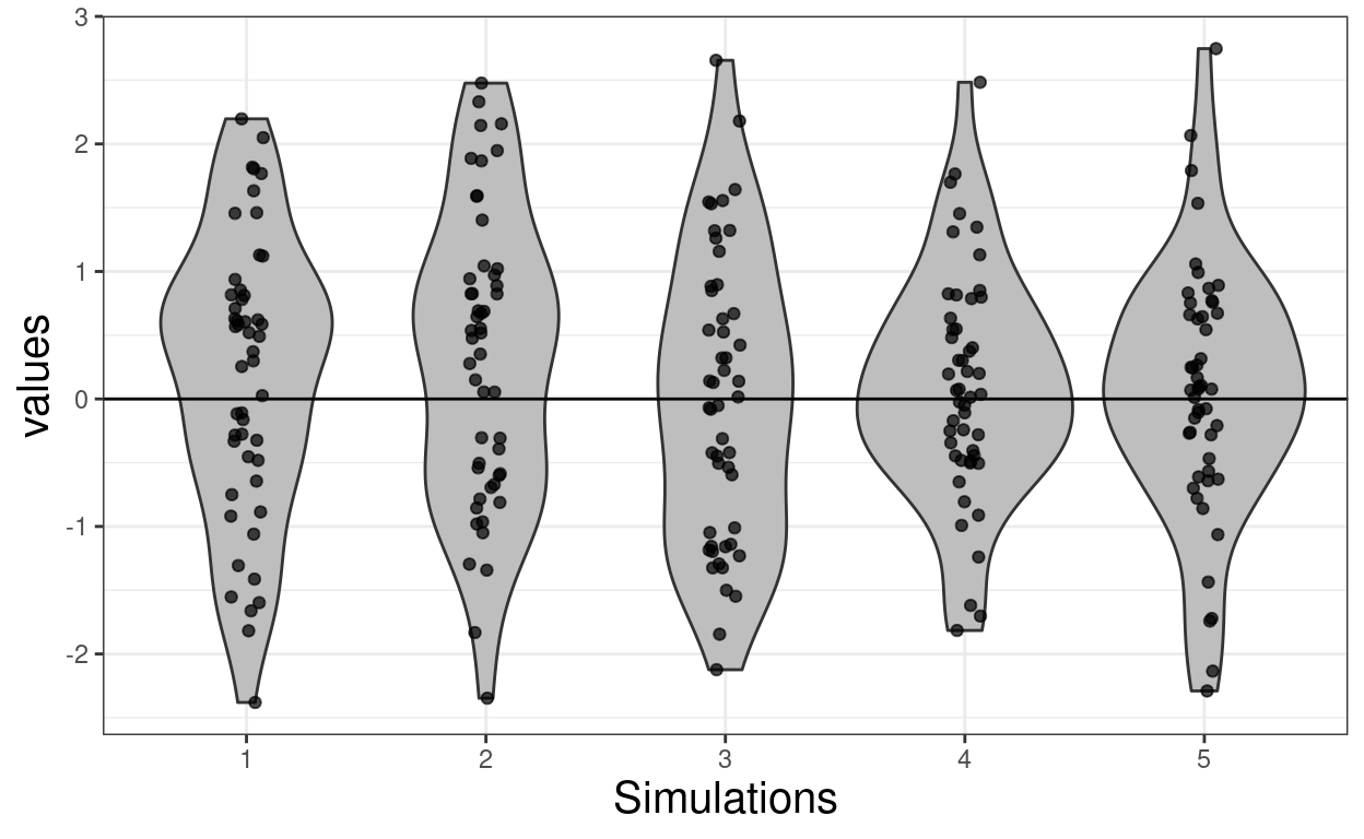
Show code
ggsave(filename = "geomViolin4.png",
       width = 1700,
       height = 1470,
       units = "px")

### now move to different sample sizes
c(50, 100, 200, 500, 1000, 5000, 50000, 500000) -> tmpVecN
### get sample sizes into human readable rather than scientific format
prettyNum(tmpVecN, big.mark = ",", scientific = FALSE) -> tmpVecLabels

tmpVecN %>%
  as_tibble() %>%
  rename(n = value) %>%
  ### need rowwise() otherwise dplyr seems to use same seed each time
  rowwise() %>%
  mutate(values = list(rnorm(n))) %>%
  ungroup() %>%
  ### applying the labels to get discrete and readable variable
  mutate(nFac = ordered(n,
                     labels = tmpVecLabels)) %>%
  unnest_longer(values) -> tmpTib

ggplot(data = tmpTib,
       aes(x = nFac, y = values)) +
  geom_violin(fill = "grey") +
  geom_jitter(height = 0, width = .1, alpha = .3) +
  geom_hline(yintercept = 0) +
  scale_x_discrete()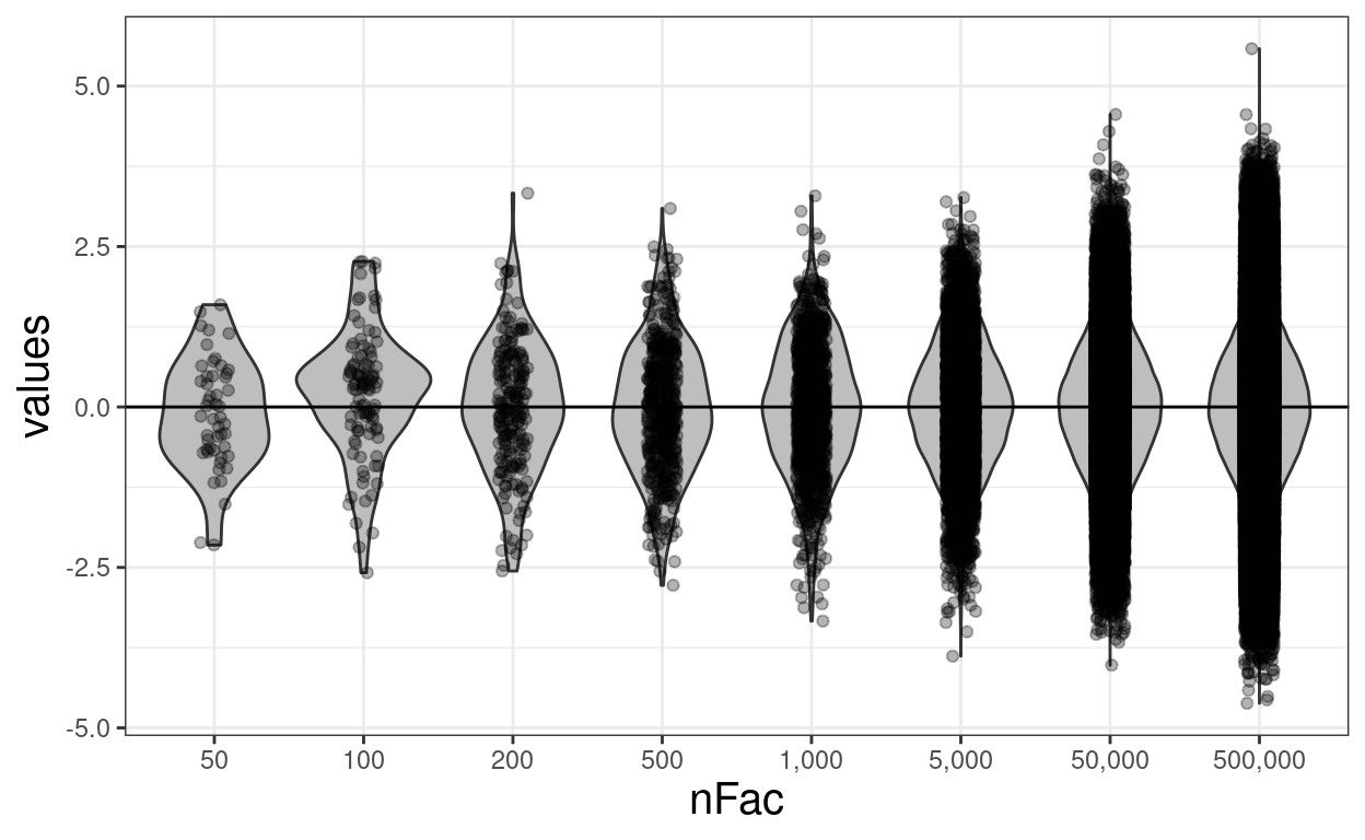
Show code
ggsave(filename = "geomViolin5.png",
       width = 1700,
       height = 1470,
       units = "px")

### but showing the points in the larger samples is mad so ...
ggplot(data = tmpTib,
       aes(x = nFac, y = values)) +
  geom_violin(fill = "grey") +
  geom_jitter(data = filter(tmpTib, n < 5000),
              height = 0, width = .15, alpha = .1) +
  geom_hline(yintercept = 0) +
  scale_x_discrete()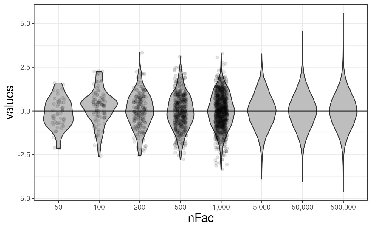
Show code
ggsave(filename = "geomViolin6.png",
       width = 1700,
       height = 1470,
       units = "px")


### now some real data
tibRawDat %>%
  filter(!is.na(SocState)) %>%
  filter(!is.na(Gender)) %>%
  mutate(SocStat2 = recode(SocStatNA,
                           "NA" = NA_character_,
                           "Divorced" = "Single",
                           "Separated" = "Single",
                           "Widowed/Widower" = "Single")) -> tmpTib

tmpTib %>%
  group_by(Gender, SocStat2) %>%
  summarise(CI = list(getBootCImean(meanCOREOM))) %>%
  unnest_wider(CI) -> tmpSummary
tmpSummary
# A tibble: 4 × 5
# Groups: Gender [2]
Gender SocStat2 obsmean LCLmean UCLmean
<chr> <chr> <dbl> <dbl> <dbl>
1 Female Coupled 0.778 0.695 0.861
2 Female Single 1.03 0.978 1.08
3 Male Coupled 0.728 0.670 0.793
4 Male Single 1.03 0.967 1.09 Show code
ggplot(data = tmpTib,
       aes(x = interaction(Gender, SocStat2), y = meanCOREOM, fill = Gender)) +
  geom_violin() +
  geom_jitter(height = 0, width = .1, alpha = .2) +
  geom_hline(yintercept = mean(tmpTib$meanCOREOM)) +
  ### add summary statistics
  geom_point(data = tmpSummary,
             aes(y = obsmean),
             position = position_nudge(x = -.15),
             size = 2.5) +
  geom_linerange(data = tmpSummary,
                 inherit.aes = FALSE,
                 aes(x = interaction(Gender, SocStat2),
                     ymin = LCLmean, ymax = UCLmean),
                 position = position_nudge(x = -.15),
                 size = 1.5) +
  xlab("Gender and social status") +
  ylab("CORE-OM score (mean item score)")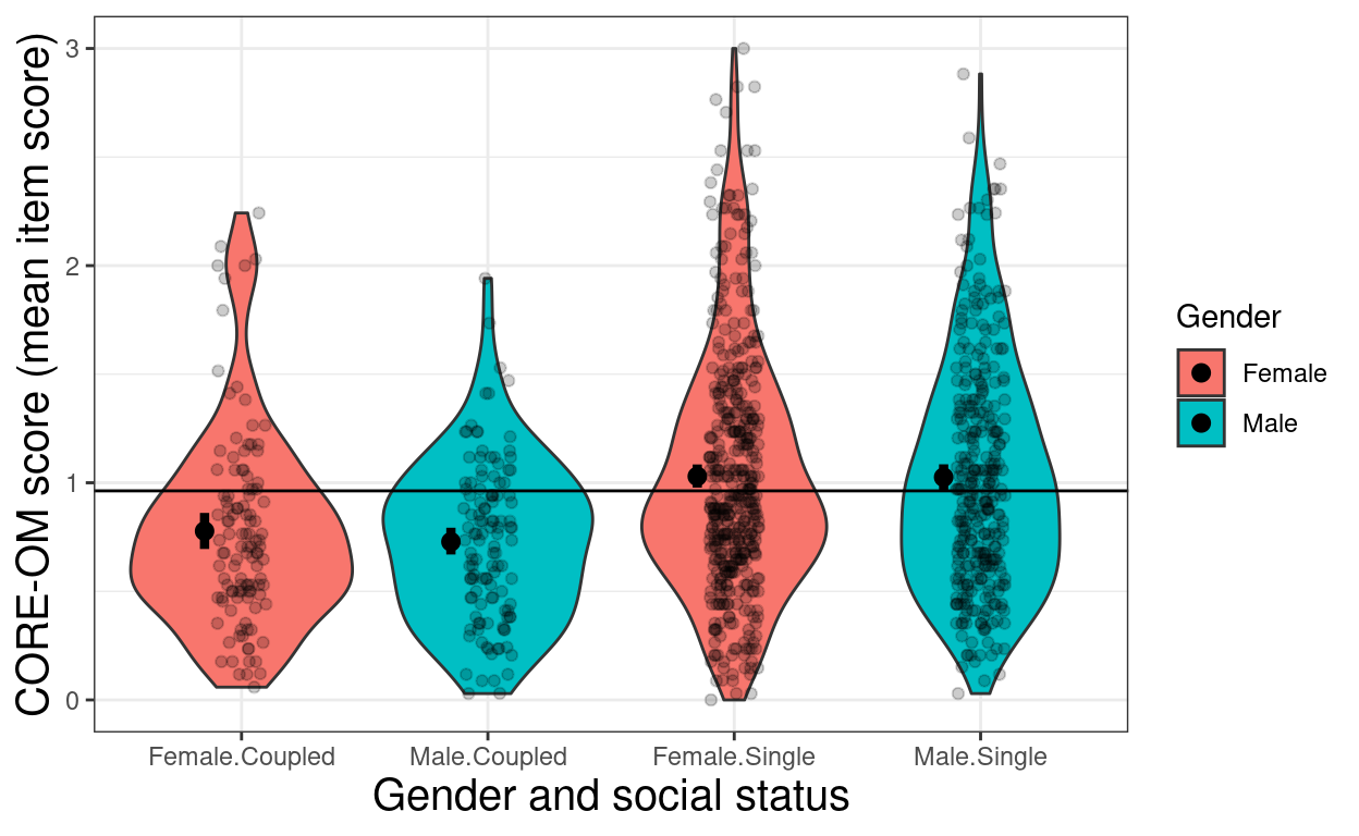
Show code
ggsave(filename = "geomViolin7.png",
       width = 1700,
       height = 1470,
       units = "px")
Show code
### get the data
tibUseDat %>%
  mutate(SocState = `Estado civil`,
         SocState = recode(SocState,
                           `Casado/a` = "Coupled",
                           `Soltero`  = "Single",
                           `Separado/a` = "Separated",
                           `Divorciado/a` = "Divorced",
                           `Unido/a` = "Coupled",
                           `Unido` = "Coupled",
                           `Viudo/a` = "Widowed/Widower")) %>%
  rowwise() %>%
  mutate(meanCOREOM = meanNotNA(c_across(COREOM01_01:COREOM01_34))) %>%
  ungroup() -> tibUseDat

### histogram of the raw data
ggplot(data = tibUseDat,
       aes(x = meanCOREOM)) +
  geom_histogram() +
  xlab("CORE-OM total score (item mean)") +
  ylab("Count")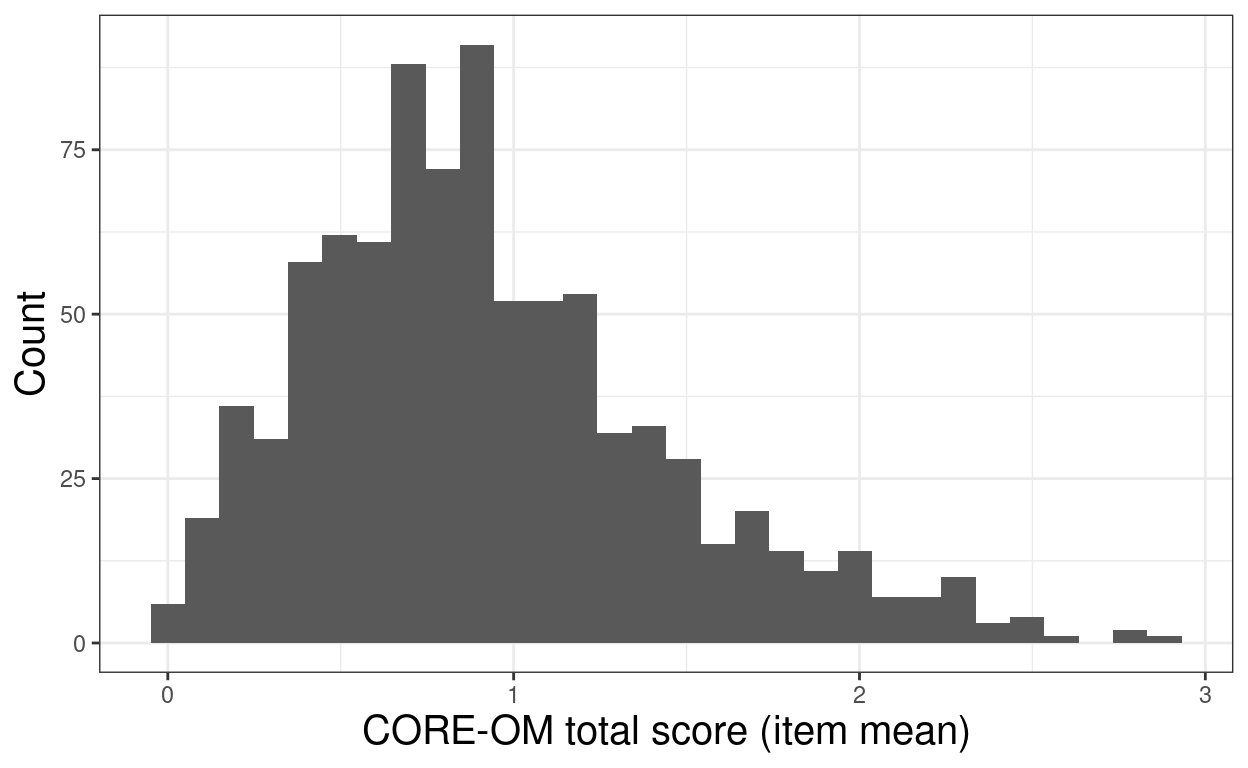
Show code
[1] 0.9312496Show code
var(tibUseDat$meanCOREOM)[1] 0.2700728Show code
sd(tibUseDat$meanCOREOM)[1] 0.5196853[1] 0.01646686[1] 0.8989745[1] 0.9635246Show code
# tibUseDat %>%
#   select(Gender, SocState, meanCOREOM) %>%
#   drop_na() -> tmpTib
#
# ggplot(data = tmpTib,
#        aes(x = Gender, y = meanCOREOM)) +
#   geom_boxplot(varwidth = TRUE, notch = TRUE)
#
# ggplot(data = tmpTib,
#        aes(x = Gender, y = meanCOREOM)) +
#   geom_violin()

### get a well validated jackknife method
bootstrap::jackknife(tmpTib$meanCOREOM, mean)
$jack.se
[1] 0.01688115
$jack.bias
[1] 0
$jack.values
[1] 0.9630860 0.9628791 0.9629973 0.9629418 0.9634407 0.9629678
[7] 0.9630564 0.9627608 0.9628809 0.9634998 0.9629086 0.9631747
[13] 0.9627904 0.9631747 0.9630564 0.9633225 0.9633225 0.9617263
[19] 0.9632338 0.9634112 0.9633986 0.9629086 0.9632929 0.9632042
[25] 0.9627608 0.9631156 0.9629382 0.9624948 0.9628200 0.9630269
[31] 0.9633816 0.9625244 0.9634703 0.9629973 0.9629973 0.9631451
[37] 0.9623327 0.9631451 0.9628495 0.9631451 0.9628495 0.9635294
[43] 0.9629382 0.9625244 0.9628791 0.9632634 0.9625835 0.9629678
[49] 0.9636181 0.9628791 0.9632634 0.9631156 0.9632042 0.9632634
[55] 0.9633682 0.9625835 0.9623766 0.9635885 0.9625835 0.9628791
[61] 0.9632929 0.9629418 0.9637954 0.9633520 0.9635885 0.9637067
[67] 0.9618149 0.9637067 0.9637067 0.9637363 0.9627608 0.9635294
[73] 0.9626722 0.9629113 0.9631451 0.9630269 0.9632338 0.9627608
[79] 0.9632634 0.9633225 0.9632042 0.9636181 0.9620810 0.9630636
[85] 0.9627017 0.9618741 0.9629113 0.9628200 0.9637336 0.9630860
[91] 0.9627904 0.9627017 0.9633816 0.9637954 0.9628791 0.9632042
[97] 0.9627608 0.9626130 0.9627904 0.9632929 0.9632929 0.9626068
[103] 0.9631451 0.9632929 0.9635294 0.9636181 0.9630269 0.9627017
[109] 0.9629770 0.9636476 0.9633225 0.9634703 0.9630860 0.9626426
[115] 0.9634998 0.9636476 0.9635590 0.9632042 0.9632634 0.9631451
[121] 0.9629678 0.9631156 0.9635885 0.9630564 0.9628200 0.9634703
[127] 0.9629382 0.9634998 0.9611055 0.9627608 0.9629382 0.9632634
[133] 0.9627017 0.9630564 0.9632338 0.9631451 0.9625835 0.9631451
[139] 0.9633225 0.9630564 0.9631451 0.9634998 0.9629678 0.9617854
[145] 0.9622879 0.9626722 0.9627904 0.9624357 0.9625835 0.9627608
[151] 0.9628791 0.9626426 0.9632634 0.9633816 0.9627904 0.9629973
[157] 0.9633816 0.9630269 0.9627608 0.9631451 0.9632929 0.9632338
[163] 0.9623766 0.9634998 0.9635590 0.9633816 0.9625835 0.9629722
[169] 0.9619036 0.9626426 0.9625539 0.9629678 0.9632929 0.9634112
[175] 0.9623561 0.9632929 0.9630269 0.9629382 0.9634407 0.9637067
[181] 0.9623174 0.9618149 0.9625539 0.9629678 0.9630860 0.9636181
[187] 0.9632929 0.9630860 0.9624948 0.9627608 0.9627017 0.9629973
[193] 0.9634112 0.9633816 0.9621992 0.9629086 0.9630860 0.9625835
[199] 0.9615785 0.9629086 0.9632929 0.9637032 0.9624948 0.9631451
[205] 0.9629973 0.9629678 0.9631156 0.9624061 0.9620219 0.9625835
[211] 0.9627608 0.9635294 0.9624357 0.9630564 0.9631747 0.9633816
[217] 0.9628495 0.9623631 0.9629276 0.9628504 0.9623661 0.9625244
[223] 0.9630860 0.9637067 0.9633225 0.9631451 0.9637954 0.9632929
[229] 0.9632042 0.9629086 0.9629382 0.9627017 0.9634703 0.9632463
[235] 0.9634900 0.9636181 0.9622109 0.9627017 0.9629973 0.9633520
[241] 0.9631451 0.9632042 0.9627608 0.9633225 0.9634703 0.9631156
[247] 0.9637067 0.9637067 0.9629382 0.9635885 0.9636476 0.9628791
[253] 0.9633520 0.9621105 0.9615785 0.9628200 0.9634703 0.9632929
[259] 0.9631747 0.9633225 0.9629382 0.9631451 0.9630564 0.9632634
[265] 0.9615785 0.9632634 0.9621105 0.9634407 0.9635885 0.9630564
[271] 0.9624948 0.9634703 0.9635885 0.9636476 0.9635590 0.9632634
[277] 0.9629973 0.9627017 0.9634703 0.9633520 0.9618741 0.9629418
[283] 0.9635590 0.9627313 0.9631451 0.9632042 0.9620219 0.9632042
[289] 0.9631451 0.9636727 0.9634998 0.9630860 0.9630880 0.9624948
[295] 0.9635813 0.9631156 0.9628809 0.9615713 0.9628809 0.9626130
[301] 0.9632634 0.9626722 0.9630564 0.9632042 0.9627591 0.9629973
[307] 0.9637363 0.9626722 0.9635813 0.9631451 0.9632929 0.9634112
[313] 0.9636181 0.9627608 0.9631747 0.9628200 0.9632634 0.9634112
[319] 0.9629382 0.9624061 0.9634998 0.9620810 0.9628791 0.9629382
[325] 0.9632042 0.9634703 0.9633520 0.9630269 0.9624652 0.9634112
[331] 0.9627608 0.9631156 0.9629678 0.9630860 0.9635590 0.9631156
[337] 0.9632929 0.9629678 0.9632929 0.9627017 0.9619332 0.9628495
[343] 0.9623766 0.9635885 0.9629722 0.9633225 0.9627608 0.9632929
[349] 0.9632042 0.9629086 0.9628495 0.9628791 0.9632634 0.9627904
[355] 0.9629678 0.9637363 0.9625539 0.9629113 0.9630564 0.9634407
[361] 0.9626130 0.9628200 0.9630860 0.9628791 0.9629382 0.9629678
[367] 0.9632042 0.9634703 0.9634998 0.9629973 0.9635294 0.9626722
[373] 0.9637659 0.9631747 0.9624948 0.9631654 0.9629113 0.9613438
[379] 0.9635590 0.9622879 0.9632042 0.9615489 0.9629382 0.9637945
[385] 0.9636118 0.9621105 0.9627608 0.9631451 0.9630269 0.9632042
[391] 0.9633225 0.9634112 0.9620219 0.9634407 0.9623022 0.9633377
[397] 0.9624061 0.9630564 0.9634112 0.9633520 0.9620586 0.9626130
[403] 0.9614307 0.9624061 0.9628791 0.9627904 0.9618741 0.9627904
[409] 0.9631747 0.9626068 0.9626130 0.9632634 0.9631451 0.9627313
[415] 0.9627017 0.9626130 0.9632929 0.9620810 0.9633225 0.9620514
[421] 0.9628495 0.9632634 0.9627608 0.9633816 0.9628200 0.9622457
[427] 0.9625835 0.9627904 0.9629678 0.9621697 0.9634703 0.9629086
[433] 0.9631747 0.9616376 0.9624357 0.9629418 0.9633225 0.9612829
[439] 0.9625835 0.9627904 0.9628495 0.9632042 0.9632042 0.9631747
[445] 0.9629973 0.9626130 0.9614898 0.9624061 0.9629086 0.9629973
[451] 0.9633816 0.9626981 0.9629722 0.9629086 0.9627017 0.9632634
[457] 0.9636181 0.9625539 0.9626130 0.9621401 0.9627904 0.9625539
[463] 0.9630564 0.9631550 0.9624948 0.9614602 0.9630860 0.9625539
[469] 0.9627017 0.9617558 0.9630269 0.9624357 0.9628200 0.9620219
[475] 0.9621992 0.9625539 0.9622879 0.9622583 0.9625835 0.9633520
[481] 0.9630860 0.9625835 0.9615785 0.9615489 0.9630564 0.9630269
[487] 0.9624948 0.9625244 0.9621992 0.9629973 0.9624061 0.9624652
[493] 0.9627313 0.9633816 0.9629086 0.9625539 0.9626722 0.9629678
[499] 0.9625835 0.9632338 0.9630636 0.9626426 0.9626130 0.9631747
[505] 0.9632929 0.9623174 0.9619923 0.9633225 0.9630564 0.9627313
[511] 0.9631245 0.9622879 0.9631451 0.9633225 0.9627608 0.9621992
[517] 0.9631156 0.9622879 0.9617854 0.9628200 0.9621992 0.9627904
[523] 0.9623766 0.9627313 0.9623174 0.9623174 0.9616967 0.9626722
[529] 0.9619036 0.9629678 0.9634703 0.9632929 0.9631451 0.9634703
[535] 0.9631747 0.9634703 0.9626426 0.9628495 0.9634407 0.9615785
[541] 0.9619332 0.9624545 0.9632634 0.9626722 0.9629086 0.9631747
[547] 0.9625835 0.9632338 0.9623174 0.9629973 0.9623470 0.9632042
[553] 0.9631156 0.9630564 0.9627313 0.9624948 0.9619627 0.9631550
[559] 0.9623022 0.9627482 0.9624652 0.9632929 0.9622879 0.9621697
[565] 0.9631156 0.9628791 0.9624061 0.9630860 0.9624357 0.9627608
[571] 0.9630860 0.9625244 0.9630564 0.9632042 0.9636772 0.9628495
[577] 0.9622879 0.9630269 0.9631747 0.9627608 0.9625539 0.9619036
[583] 0.9625244 0.9624652 0.9617854 0.9616931 0.9629973 0.9634703
[589] 0.9615104 0.9628809 0.9625835 0.9623470 0.9619332 0.9628495
[595] 0.9618445 0.9632463 0.9616671 0.9626722 0.9624948 0.9620810
[601] 0.9615489 0.9621992 0.9624745 0.9627904 0.9623766 0.9626722
[607] 0.9621992 0.9624652 0.9628791 0.9629678 0.9620890 0.9631747
[613] 0.9617263 0.9635885 0.9631451 0.9629973 0.9632338 0.9623470
[619] 0.9626426 0.9627904 0.9628200 0.9633520 0.9627608 0.9622288
[625] 0.9627608 0.9630269 0.9629678 0.9632929 0.9633816 0.9630269
[631] 0.9634407 0.9632338 0.9623936 0.9620810 0.9635885 0.9632634
[637] 0.9630564 0.9625244 0.9628495 0.9625835 0.9635885 0.9633816
[643] 0.9636476 0.9629382 0.9624652 0.9624652 0.9623174 0.9616080
[649] 0.9634998 0.9634703 0.9629678 0.9615193 0.9627608 0.9632338
[655] 0.9632338 0.9631156 0.9632042 0.9632929 0.9631156 0.9626426
[661] 0.9634112 0.9627608 0.9620810 0.9618149 0.9629382 0.9629973
[667] 0.9623470 0.9630860 0.9636772 0.9627608 0.9635294 0.9625244
[673] 0.9631156 0.9632338 0.9630860 0.9633520 0.9635885 0.9630564
[679] 0.9627017 0.9627017 0.9638250 0.9633520 0.9633225 0.9632042
[685] 0.9623470 0.9633986 0.9633816 0.9633225 0.9628495 0.9628791
[691] 0.9626130 0.9629973 0.9625244 0.9626722 0.9628200 0.9635885
[697] 0.9633816 0.9616671 0.9628504 0.9629086 0.9617263 0.9630636
[703] 0.9629418 0.9633816 0.9623936 0.9624652 0.9633520 0.9634407
[709] 0.9618741 0.9624948 0.9626426 0.9636181 0.9628791 0.9614898
[715] 0.9613715 0.9621105 0.9631156 0.9630860 0.9623470 0.9624948
[721] 0.9619332 0.9631451 0.9619332 0.9634112 0.9634998 0.9631451
[727] 0.9632338 0.9615785 0.9621401 0.9634407 0.9630564 0.9626426
[733] 0.9622879 0.9612829 0.9637954 0.9629382 0.9627904 0.9621401
[739] 0.9636772 0.9634900 0.9636181 0.9633520 0.9630564 0.9627591
[745] 0.9632634 0.9629382 0.9633816 0.9625835 0.9617558 0.9630564
[751] 0.9631747 0.9635885 0.9612829 0.9631747 0.9627017 0.9630269
[757] 0.9627017 0.9634112 0.9622583 0.9634112 0.9631854 0.9629382
[763] 0.9634407 0.9631451 0.9636181 0.9628200 0.9632042 0.9615489
[769] 0.9631156 0.9631747 0.9623766 0.9633816 0.9627904 0.9628791
[775] 0.9630860 0.9627608 0.9626426 0.9622288 0.9632042 0.9630269
[781] 0.9615489 0.9630860 0.9631747 0.9632929 0.9629382 0.9632929
[787] 0.9628495 0.9628495 0.9632042 0.9630269 0.9627608 0.9631156
[793] 0.9630941 0.9626426 0.9619332 0.9628495 0.9624357 0.9633225
[799] 0.9619627 0.9629086 0.9634703 0.9630269 0.9634703 0.9623766
[805] 0.9625539 0.9630860 0.9624948 0.9630269 0.9629678 0.9634998
[811] 0.9628495 0.9619627 0.9630564 0.9622288 0.9625244 0.9618454
[817] 0.9629973 0.9635294 0.9618741 0.9625539 0.9629086 0.9627313
[823] 0.9630564 0.9633816 0.9627017 0.9633225 0.9629973 0.9625539
[829] 0.9629973 0.9628791 0.9610464 0.9623470 0.9609873 0.9624357
[835] 0.9619923 0.9632634 0.9615713 0.9620219 0.9628791 0.9624061
[841] 0.9629678 0.9614602 0.9624357 0.9628791 0.9629678 0.9629382
[847] 0.9630860 0.9623470 0.9619923 0.9629678 0.9622879 0.9631451
[853] 0.9637363 0.9627904 0.9631747 0.9626068 0.9635590 0.9634998
[859] 0.9632338 0.9629142 0.9628809 0.9626130 0.9629418 0.9629086
[865] 0.9627904 0.9632634 0.9621697 0.9625244 0.9629382 0.9627904
[871] 0.9631451 0.9630564 0.9626130 0.9632042 0.9619672 0.9631747
[877] 0.9614602 0.9621697 0.9630564 0.9629678 0.9627904 0.9629973
[883] 0.9633520 0.9608099 0.9629678 0.9627608 0.9634595 0.9628791
[889] 0.9631451 0.9624357 0.9627904 0.9625835 0.9630860 0.9633520
[895] 0.9621992 0.9619332 0.9625244 0.9630564 0.9628495 0.9621697
[901] 0.9636476 0.9621697 0.9630564 0.9625244 0.9629382 0.9625154
[907] 0.9625835 0.9617558 0.9628495 0.9620810 0.9618741 0.9625244
[913] 0.9629973 0.9629678 0.9633520 0.9623470 0.9633225 0.9630269
[919] 0.9633225 0.9630860 0.9628495 0.9628200 0.9631747 0.9626130
[925] 0.9636476 0.9629086 0.9628200 0.9620219 0.9632929 0.9617263
[931] 0.9620219 0.9627608 0.9622879 0.9636772 0.9630269 0.9628791
[937] 0.9623174 0.9609873 0.9626426 0.9628495 0.9631451 0.9634998
[943] 0.9637363 0.9636181 0.9631156 0.9630564 0.9630269 0.9633816
[949] 0.9635590 0.9633520 0.9625835 0.9624652 0.9621992 0.9622583
[955] 0.9624061 0.9632042 0.9631451 0.9629382 0.9624357 0.9633816
[961] 0.9617854 0.9629086 0.9627904 0.9632929 0.9636476 0.9629456
[967] 0.9627608 0.9627313 0.9629973 0.9625835 0.9626981 0.9622839
[973] 0.9627313 0.9629086 0.9634998 0.9618149 0.9609281 0.9629382
[979] 0.9625835 0.9623470 0.9624061 0.9626722 0.9625835 0.9619923
[985] 0.9626426 0.9622879 0.9614898 0.9614602 0.9633816 0.9632634
[991] 0.9630860 0.9620219 0.9632338 0.9631747 0.9630398 0.9612237
$call
bootstrap::jackknife(x = tmpTib$meanCOREOM, theta = mean)Show code
### but I'm a masochistic, obsessional idiot so I replicate that!
jackMean <- function(x, confint = .95){
  x <- na.omit(x)
  valN <- length(x)
  valSampMean <- mean(x)
  vecJackMeans <- rep(NA, valN)
  vecPseudoVals <- rep(NA, valN)

  for (i in 1:valN){
    vecJackMeans[i] <- mean(x[-i])
    vecPseudoVals[i] <- valN * valSampMean - (valN - 1)*vecJackMeans[i]
  }
  valBias <- (valN - 1) * (mean(vecJackMeans) - valSampMean)
  valSE <- sqrt(((valN - 1) / valN) * sum((vecJackMeans - mean(vecJackMeans))^2))
  valQt <- qt((1 - (1 - confint)/2), valN - 1)
  print(valQt)
  LCL <- valSampMean - (valSE * valQt)
  UCL <- valSampMean + (valSE * valQt)
  return(list(n = valN,
              mean = valSampMean,
              bias = valBias,
              SE = valSE,
              confint = confint,
              LCL = LCL,
              UCL = UCL,
              CI = c(LCL, UCL),
              vecJackMeans = vecJackMeans,
              vecPseudoVals = vecPseudoVals))
}

# jackMean(1:8)
# bootstrap::jackknife(1:8, mean)

jackMean(tmpTib$meanCOREOM) -> listJackknife
[1] 1.962351Show code
bootstrap::jackknife(tmpTib$meanCOREOM, mean)$jack.bias[1] 0Show code
bootstrap::jackknife(tmpTib$meanCOREOM, mean)$jack.se[1] 0.01688115Show code
listJackknife$bias[1] 0Show code
listJackknife$SE[1] 0.01688115Show code
listJackknife$CI[1] 0.9297305 0.9959840Show code
range(listJackknife$vecJackMeans)[1] 0.9608099 0.9638250[1] 0.9628573Show code
mean(tmpTib$meanCOREOM)[1] 0.9628573Show code
ggplot(data = tmpTibJackknife,
       aes(x = value)) +
  geom_histogram() +
  geom_vline(xintercept = mean(tmpTibJackknife$value),
             colour = "green",
             size = 2) +
  xlab("Jackknife means") +
  ylab("Count")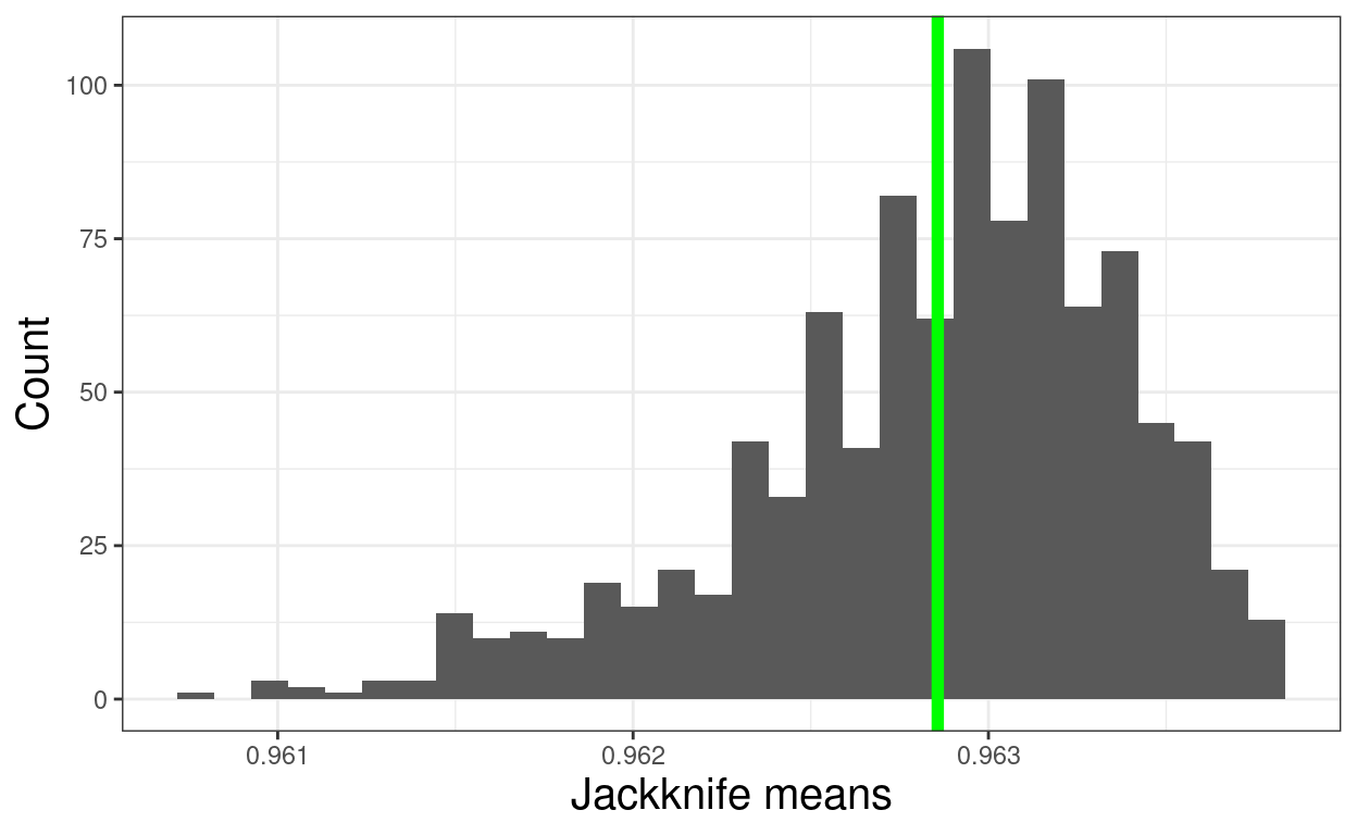
Show code
ggsave(filename = "jackknife2.png",
       width = 1700,
       height = 1470,
       units = "px")


### create an evenly spread small subsample
tmpTib %>%
  arrange(meanCOREOM) %>%
  mutate(rowN = row_number()) %>%
  filter(rowN %% 20 == 10) -> tmpTib2
# max(tmpTib2$rowN)
# nrow(tmpTib2)

ggplot(data = tmpTib2,
       aes(x = meanCOREOM)) +
  geom_histogram() +
  xlab("CORE-OM total score (item mean)") +
  ylab("Count")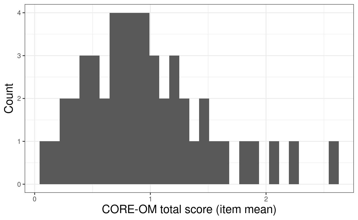
Show code
[1] 0.9687147Show code
var(tmpTib2$meanCOREOM)[1] 0.296774[1] 0.01726169[1] 0.8177122[1] 1.119717Show code
### jackknifing
jackMean(tmpTib2$meanCOREOM) -> listJackknife2
[1] 2.009575Show code
bootstrap::jackknife(tmpTib2$meanCOREOM, mean)$jack.bias[1] 0Show code
bootstrap::jackknife(tmpTib2$meanCOREOM, mean)$jack.se[1] 0.07704206Show code
listJackknife2$bias[1] 0Show code
listJackknife2$SE[1] 0.07704206Show code
listJackknife2$CI[1] 0.8138928 1.1235365Show code
range(listJackknife2$vecJackMeans)[1] 0.9356632 0.9866836Show code
listJackknife2$vecJackMeans %>%
  as_tibble() -> tmpTibJackknife2

ggplot(data = tmpTibJackknife2,
       aes(x = value)) +
  geom_histogram() +
  geom_vline(xintercept = mean(tmpTibJackknife$value),
             colour = "green",
             size = 2) +
  xlab("Jackknife means") +
  ylab("Count")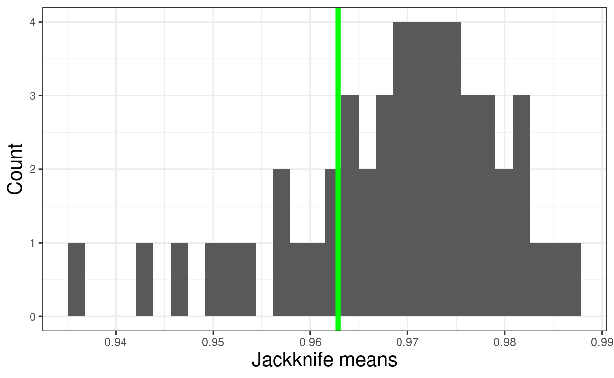
Show code
ggsave(filename = "jackknife4.png",
       width = 1700,
       height = 1470,
       units = "px")
Show code
Time difference of 0.3149319 secsShow code
[1] 0.8807916 1.0319069Show code
mean(tmpTibBoot$value)[1] 0.9630155Show code
tmpRes$t0[1] 0.9628573Show code
ggplot(data = tmpTibBoot,
       aes(x = value)) +
  geom_histogram() +
  geom_vline(xintercept = mean(tmpTibBoot$value),
             colour = "green",
             size = 3.5) +
  geom_vline(xintercept = mean(tmpTib$meanCOREOM),
             colour = "blue")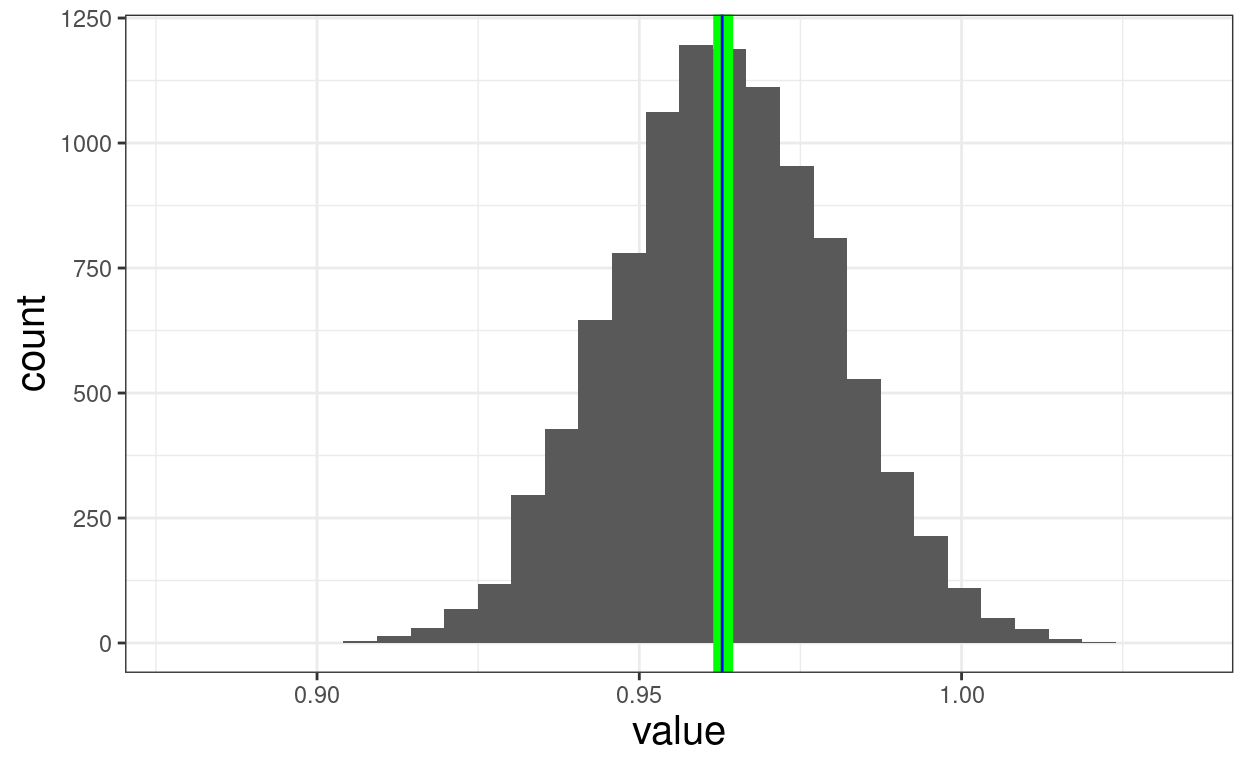
Show code
ggsave(filename = "bootstrap1.png",
       width = 1700,
       height = 1470,
       units = "px")

tmpRes$t0
[1] 0.9628573Show code
boot::boot.ci(tmpRes)BOOTSTRAP CONFIDENCE INTERVAL CALCULATIONS
Based on 10000 bootstrap replicates
CALL :
boot::boot.ci(boot.out = tmpRes)
Intervals :
Level Normal Basic
95% ( 0.9292, 0.9962 ) ( 0.9293, 0.9954 )
Level Percentile BCa
95% ( 0.9303, 0.9964 ) ( 0.9304, 0.9965 )
Calculations and Intervals on Original ScaleShow code
Time difference of 0.08940196 secsShow code
[1] 0.7056996 1.2611440Show code
ggplot(data = tmpTibBoot,
       aes(x = value)) +
  geom_histogram() +
  geom_vline(xintercept = mean(tmpTibBoot$value),
             colour = "green",
             size = 3.5) +
  geom_vline(xintercept = mean(tmpTib$meanCOREOM),
             colour = "blue",
             size = 2)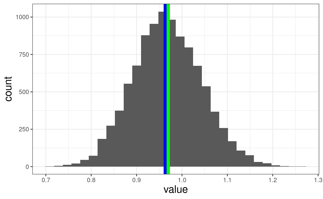
Show code
ggsave(filename = "bootstrap2.png",
       width = 1700,
       height = 1470,
       units = "px")

tmpRes$t0
[1] 0.9687147Show code
boot::boot.ci(tmpRes)BOOTSTRAP CONFIDENCE INTERVAL CALCULATIONS
Based on 10000 bootstrap replicates
CALL :
boot::boot.ci(boot.out = tmpRes)
Intervals :
Level Normal Basic
95% ( 0.8214, 1.1181 ) ( 0.8157, 1.1128 )
Level Percentile BCa
95% ( 0.8246, 1.1217 ) ( 0.8347, 1.1363 )
Calculations and Intervals on Original ScaleShow code
tribble(~DNA, ~Gender, ~n,
        "All", "F", 125,
        "All", "M", 125,
        "DNA...", "F", 125,
        "DNA...", "M", 125) -> tibAssoc125
tibAssoc125 %>%
  uncount(n) -> tibAssoc125long

### good old fashioned, well hybrid, way to do this
tibAssoc125long %>%
  summarise(chisq = list(unlist(chisq.test(Gender, DNA)))) %>%
  unnest_wider(chisq)
# A tibble: 1 × 21
`statistic.X-squared` parameter.df p.value method data.name
<chr> <chr> <chr> <chr> <chr>
1 0 1 1 Pearson's Chi-… Gender a…
# ℹ 16 more variables: observed1 <chr>, observed2 <chr>,
# observed3 <chr>, observed4 <chr>, expected1 <chr>,
# expected2 <chr>, expected3 <chr>, expected4 <chr>,
# residuals1 <chr>, residuals2 <chr>, residuals3 <chr>,
# residuals4 <chr>, stdres1 <chr>, stdres2 <chr>, stdres3 <chr>,
# stdres4 <chr>Show code
### let's see if I can get to understand the purrr and broom approach
tibAssoc125long %>%
  ### nest() makes all the data into a row with a dataframe in it of all the data
  ### have to use "data = everything" when not using it after group_by() so it knows to use all columns
  nest(data = everything()) %>%
  ### so now we have a single row tibble so mutate() not summarise()
  ### this says apply chisq.test to the data computing the chisq.test for Gender and DNA
  ### this seems horrible syntax to me
  mutate(chisq = purrr::map(data, ~chisq.test(.$Gender, .$DNA)),
         ### this is similar: apply broom::tidy() to all of chisq
         ### broom::tidy actually uses tidy.htest() seeing that chisq is an htest list
         ### so it pulls the elements into a list
         tidied = purrr::map(chisq, broom::tidy)) %>%
  ### at this point you've still got all the data in a column data
  ### and all the output of chisq.test() as a list
  ### don't need all that!
  select(tidied) %>%
  ### now unnest the elements of tidied
  unnest_wider(tidied)
# A tibble: 1 × 4
statistic p.value parameter method
<dbl> <dbl> <int> <chr>
1 0 1 1 Pearson's Chi-squared testShow code
### this was part of my abortive attempt to create tables I could easily
### paste into WordPress by making them into jpegs or pngs using tools
### it gridExtra.  I didn't crack it!
# tt3 <- ttheme_default(core=list(fg_params=list(hjust=0, x=0.1)),
#                       rowhead=list(fg_params=list(hjust=0, x=0)))
# tibAssoc125long %>%
#   tabyl(DNA, Gender) %>%
#   as.data.frame() -> tmpDF
#
#
# gridExtra::tableGrob(tmpDF, rows = NULL) -> tmpGrob
# png("test.png", height=1000, width=200)
# gridExtra::grid.table(tmpDF, rows = NULL)
# dev.off()
Show code
### trying to shift tables to WordPress using csv and the wpDataTables plugin
### recode to long labels
tibAssoc125long %>%
  mutate(DNA = recode(DNA,
                      "All" = "Attended all sessions",
                      "DNA..." = "DNAed at least one session")) -> tibAssoc125long

### simplest xtab
tibAssoc125long %>%
  tabyl(DNA, Gender)  %>%
  ### get top left cell correct
  rename(n = DNA) %>%
  write_csv(file = "xtab1.csv")

### simplest xtab
tibAssoc125long %>%
  tabyl(DNA, Gender)  %>%
  ### get top left cell correct
  rename(n = DNA) %>%
  flextable::flextable() %>%
  flextable::autofit() %>%
  flextable::save_as_image(path = "xtab1.png", zoom = 3)
[1] "xtab1.png"Show code
### row percentages: CSV
tibAssoc125long %>%
  tabyl(DNA, Gender)  %>%
  ### get top left cell correct
  rename(`n (row %)` = DNA) %>%
  adorn_totals(where = c("row", "col")) %>%
  adorn_percentages(denominator = "row") %>%
  adorn_pct_formatting(digits = 1) %>%
  adorn_ns(position = "front") %>%
  write_csv(file = "xtab2.csv")

### row percentages: png
tibAssoc125long %>%
  tabyl(DNA, Gender)  %>%
  ### get top left cell correct
  rename(`n (row %)` = DNA) %>%
  adorn_totals(where = c("row", "col")) %>%
  adorn_percentages(denominator = "row") %>%
  adorn_pct_formatting(digits = 1) %>%
  adorn_ns(position = "front") %>%
  flextable::flextable() %>%
  flextable::autofit() %>%
  flextable::save_as_image(path = "xtab1rowperc.png", zoom = 3)
[1] "xtab1rowperc.png"Show code
### col percentages
tibAssoc125long %>%
  tabyl(DNA, Gender)  %>%
  ### get top left cell correct
  rename(`n (col %)` = DNA) %>%
  adorn_totals(where = c("row", "col")) %>%
  adorn_percentages(denominator = "col") %>%
  adorn_pct_formatting(digits = 1) %>%
  adorn_ns(position = "front") %>%
  write_csv(file = "xtab3.csv")

### total percentages
tibAssoc125long %>%
  tabyl(DNA, Gender)  %>%
  ### get top left cell correct
  rename(`n (% of total)` = DNA) %>%
  adorn_totals(where = c("row", "col")) %>%
  adorn_percentages(denominator = "all") %>%
  adorn_pct_formatting(digits = 1) %>%
  adorn_ns(position = "front") %>%
  write_csv(file = "xtab4.csv")
Show code
vecCOREwbItems <- c(4,14,17,31)
vecCOREprobItems <- c(2,5,8,11,13,15,18,20,23,27,28,30)
vecCOREfuncItems <- c(1,3,7,10,12,19,21,25,26,29,32,33)
vecCOREriskItems <- c(6,9,16,22,24,34)
vecCOREnrItems <- c(vecCOREwbItems, vecCOREprobItems, vecCOREfuncItems)

vecCOREwbItems <- str_c("COREOM01_", sprintf("%02.0f", vecCOREwbItems))
vecCOREprobItems <- str_c("COREOM01_", sprintf("%02.0f", vecCOREprobItems))
vecCOREfuncItems <- str_c("COREOM01_", sprintf("%02.0f", vecCOREfuncItems))
vecCOREriskItems <- str_c("COREOM01_", sprintf("%02.0f", vecCOREriskItems))
vecCOREnrItems <- str_c("COREOM01_", sprintf("%02.0f", vecCOREnrItems))

tibUseDat %>%
  rowwise() %>%
  mutate(meanCOREwb = meanNotNA(c_across(all_of(vecCOREwbItems))),
         meanCOREprob = meanNotNA(c_across(all_of(vecCOREprobItems))),
         meanCOREfunc = meanNotNA(c_across(all_of(vecCOREfuncItems))),
         meanCORErisk = meanNotNA(c_across(all_of(vecCOREriskItems))),
         meanCOREnr = meanNotNA(c_across(all_of(vecCOREnrItems))),) %>%
  ungroup() -> tibUseDat


### had too much overprinting with the full dataset so:
set.seed(12345)
tibUseDat %>%
  ### my first ever use of slice_sample(): nice
  slice_sample(n = 88) -> tibSmallDat

ggplot(data = tibSmallDat,
       aes(x = meanCOREnr, y = meanCORErisk)) +
  geom_point() +
  xlab("CORE-OM non-risk score (mean item score)") +
  ylab("CORE-OM risk score (mean item score)") +
  coord_fixed(ratio = 1) +
  xlim(c(0, 4)) +
  ylim(c(0, 4))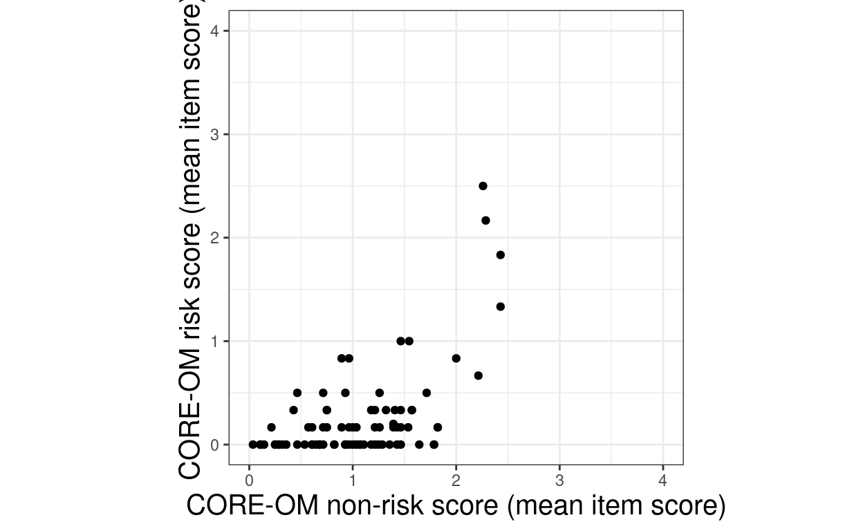
Show code
ggsave(filename = "scatterpoint.png",
       width = 1700,
       height = 1700,
       units = "px")

ggplot(data = tibSmallDat,
       aes(x = meanCOREnr, y = meanCORErisk, colour = Gender, fill = Gender)) +
  geom_point() +
  xlab("CORE-OM non-risk score (mean item score)") +
  ylab("CORE-OM risk score (mean item score)") +
  coord_fixed(ratio = 1) +
  xlim(c(0, 4)) +
  ylim(c(0, 4))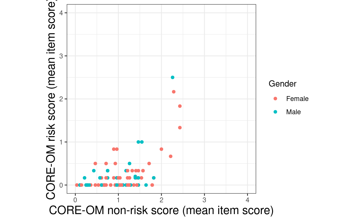
Show code
# A tibble: 1 × 1
  `n()`
  <int>
1   346
Show code
# A tibble: 148 × 3
   meanCOREnr meanCORErisk     n
        <dbl>        <dbl> <int>
 1      0.643        0        19
 2      0.536        0        16
 3      0.429        0        14
 4      0.75         0        14
 5      0.607        0        13
 6      0.679        0        13
 7      1.07         0        13
 8      0.286        0        12
 9      0.393        0        12
10      0.893        0.167    12
# ℹ 138 more rows
Show code
ggplot(data = tibUseDat,
       aes(x = meanCOREnr, y = meanCORErisk)) +
  geom_point() +
  xlab("CORE-OM non-risk score (mean item score)") +
  ylab("CORE-OM risk score (mean item score)") +
  coord_fixed(ratio = 1) +
  xlim(c(0, 4)) +
  ylim(c(0, 4))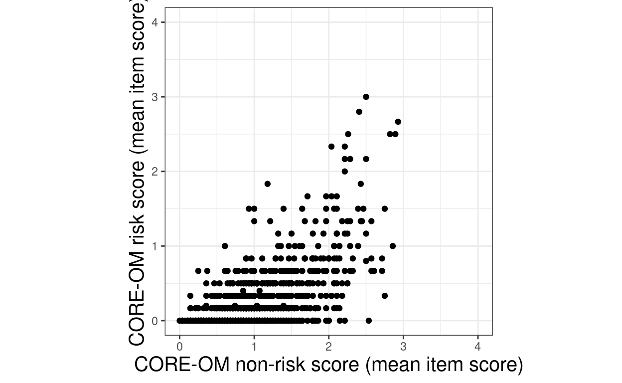
Show code
ggsave(filename = "scatter1point.png",
       width = 1700,
       height = 1700,
       units = "px")

ggplot(data = tibUseDat,
       aes(x = meanCOREnr, y = meanCORErisk)) +
  geom_point(alpha = .1) +
  xlab("CORE-OM non-risk score (mean item score)") +
  ylab("CORE-OM risk score (mean item score)") +
  coord_fixed(ratio = 1) +
  xlim(c(0, 4)) +
  ylim(c(0, 4))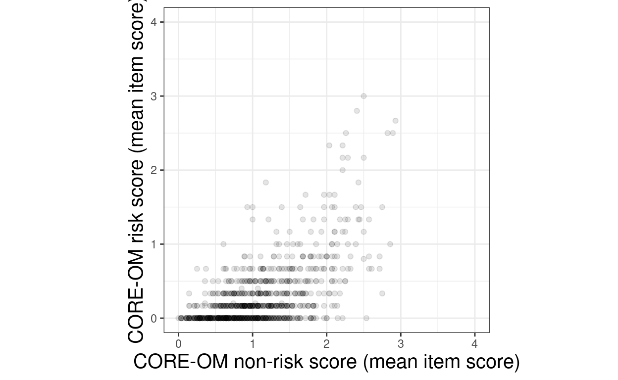
Show code
ggsave(filename = "scatter1pointAlph.png",
       width = 1700,
       height = 1700,
       units = "px")

ggplot(data = tibUseDat,
       aes(x = meanCOREnr, y = meanCORErisk)) +
  geom_count() +
  xlab("CORE-OM non-risk score (mean item score)") +
  ylab("CORE-OM risk score (mean item score)") +
  coord_fixed(ratio = 1) +
  xlim(c(0, 4)) +
  ylim(c(0, 4))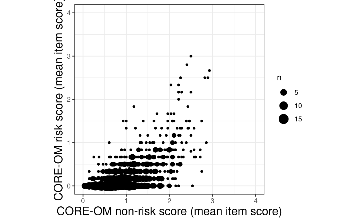
Show code
ggsave(filename = "scatter2count.png",
       width = 1700,
       height = 1700,
       units = "px")

ggplot(data = tibUseDat,
       aes(x = meanCOREnr, y = meanCORErisk)) +
  geom_count(alpha = .3) +
  xlab("CORE-OM non-risk score (mean item score)") +
  ylab("CORE-OM risk score (mean item score)") +
  coord_fixed(ratio = 1) +
  xlim(c(0, 4)) +
  ylim(c(0, 4))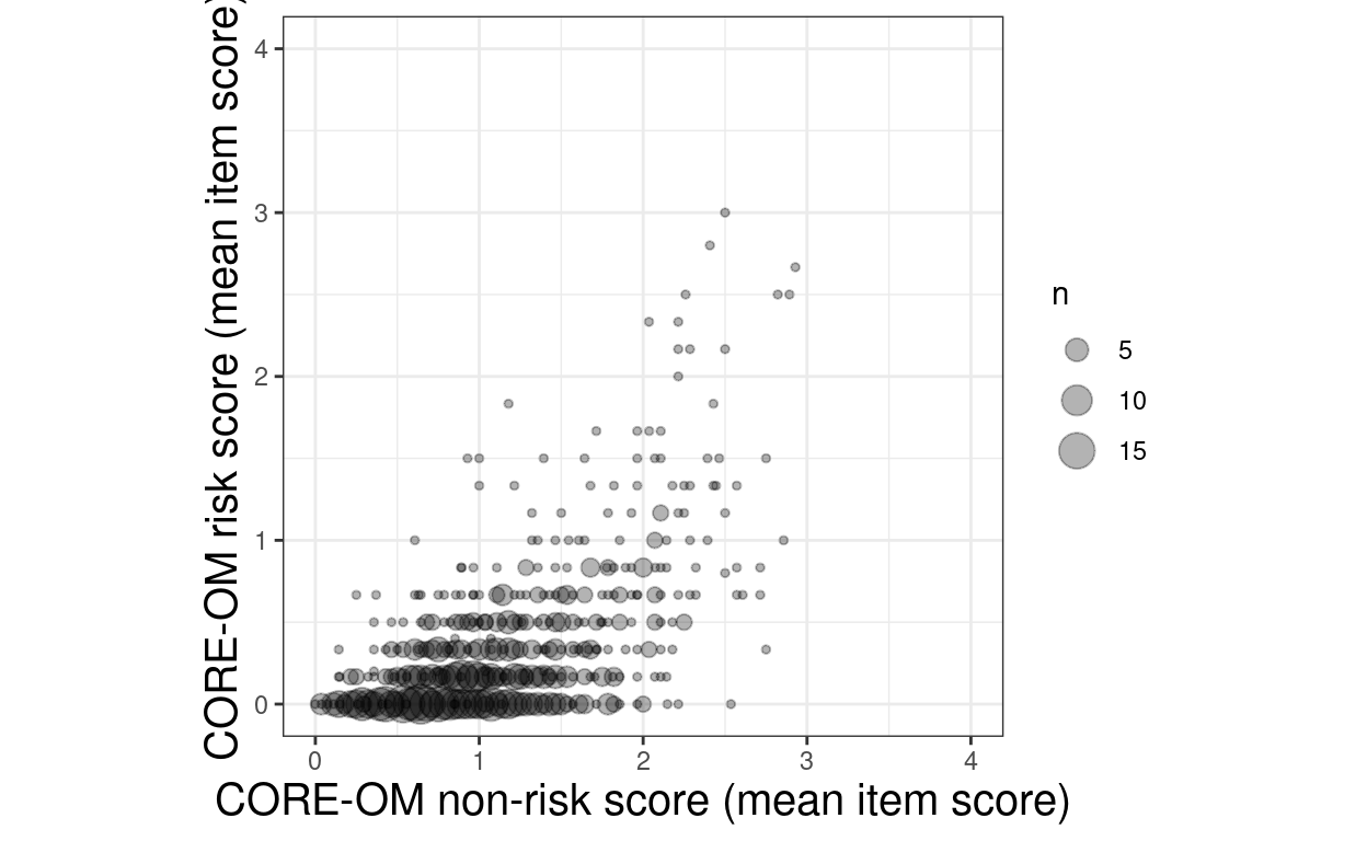
Show code
ggsave(filename = "scatter3count.png",
       width = 1700,
       height = 1700,
       units = "px")
Show code
set.seed(12345)
ggplot(data = tibUseDat,
       aes(x = meanCOREnr, y = meanCORErisk)) +
  # geom_point(colour = "blue", alpha = .2) +
  geom_jitter(width = 0, height = .05, alpha = .2) +
  xlab("CORE-OM non-risk score (mean item score)") +
  ylab("CORE-OM risk score (mean item score)") +
  coord_fixed(ratio = 1) +
  xlim(c(0, 4)) +
  ylim(c(0, 4))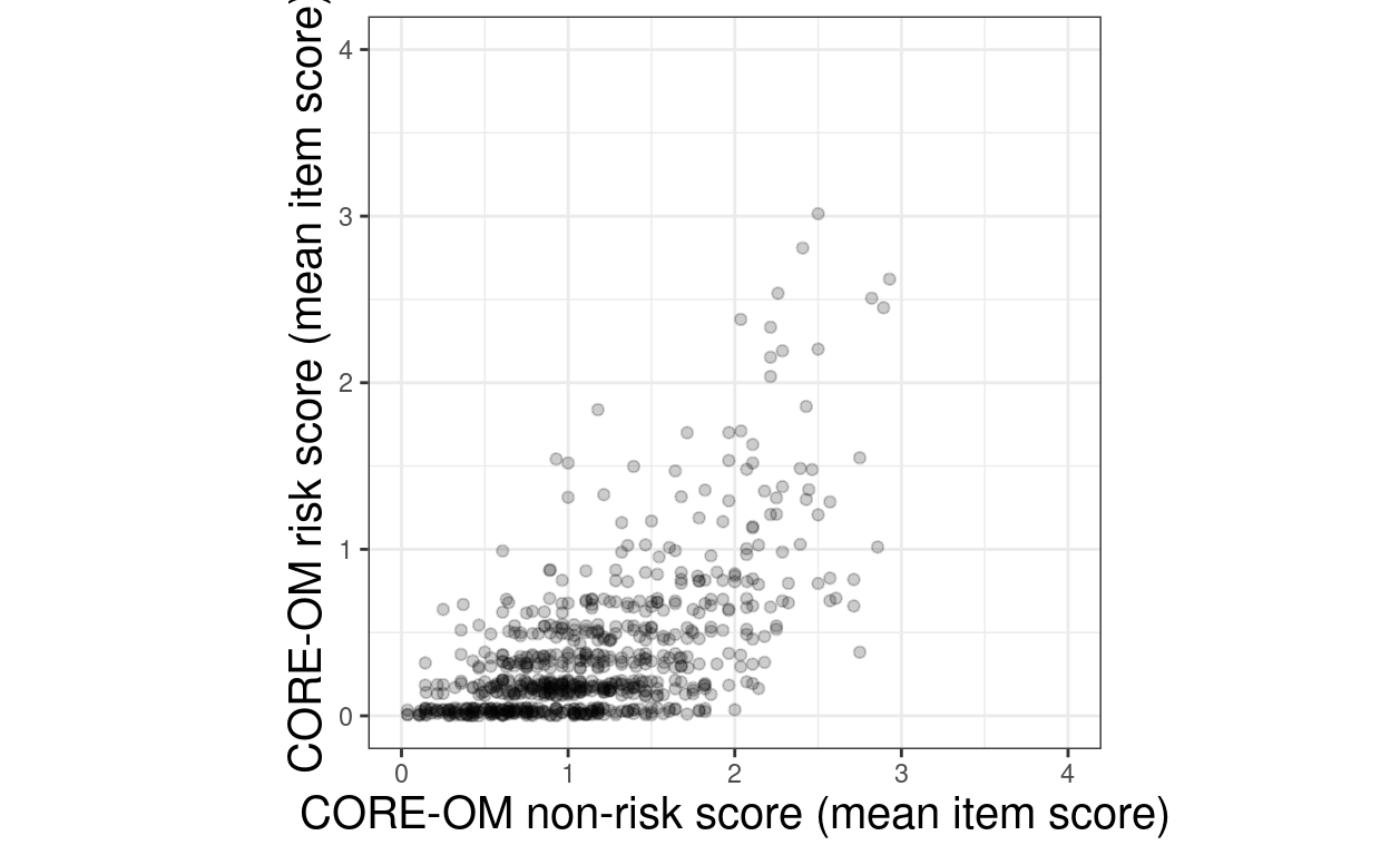
Show code
ggsave(filename = "jitter1.png",
       width = 1700,
       height = 1700,
       units = "px")

tibUseDat %>%
  # select(starts_with("COREOM01_")) %>%
  # select(-COREOM01_35) %>%
  select(all_of(vecCOREriskItems)) %>%
  na.omit() %>%
  pivot_longer(everything()) %>%
  group_by(name) %>%
  summarise(var = var(value)) %>%
  arrange(desc(var)) %>%
  slice_head()
# A tibble: 1 × 2
name var
<chr> <dbl>
1 COREOM01_06 0.591Show code
# A tibble: 1 × 2
  name          var
  <chr>       <dbl>
1 COREOM01_27  1.65
Show code
ggplot(data = tibUseDat,
       aes(x =  COREOM01_27, y = COREOM01_06)) +
  geom_point() +
  xlab("Scores on CORE-OM item 27:\nI have felt unhappy") +
  ylab("Scores on CORE-OM item 6:\nI have been physically violent to others")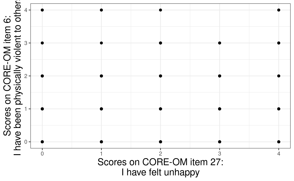
Show code
ggsave(filename = "items27and6_plot1.png",
       width = 1700,
       height = 1700,
       units = "px")

set.seed(12345)
ggplot(data = tibUseDat,
       aes(x =  COREOM01_27, y = COREOM01_06)) +
  geom_jitter(width = .4, height = .4) +
  xlab("Scores on CORE-OM item 27:\nI have felt unhappy") +
  ylab("Scores on CORE-OM item 6:\nI have been physically violent to others")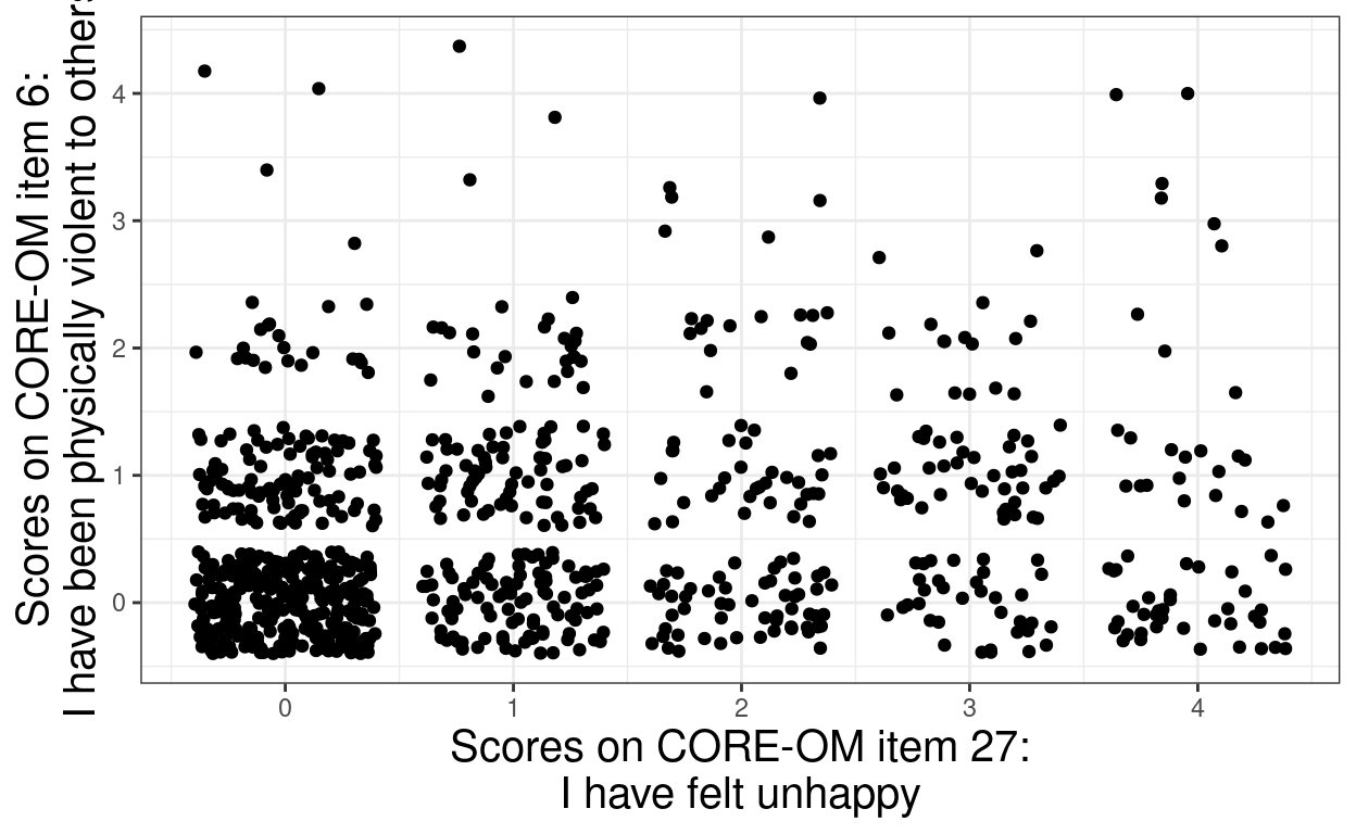
Show code
ggsave(filename = "items27and6_jitter1.png",
       width = 1700,
       height = 1700,
       units = "px")


set.seed(12345)
ggplot(data = tibUseDat,
       aes(x =  COREOM01_27, y = COREOM01_06)) +
  geom_jitter(width = .4, height = .4, alpha = .3) +
  xlab("Scores on CORE-OM item 27:\nI have felt unhappy") +
  ylab("Scores on CORE-OM item 6:\nI have been physically violent to others")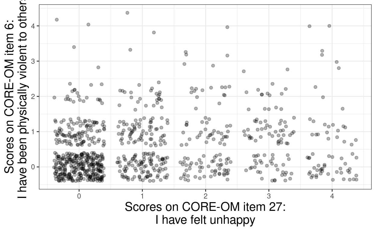
Show code
ggsave(filename = "items27and6_jitter2.png",
       width = 1700,
       height = 1700,
       units = "px")
Bits for entry about transformations
Show code
set.seed(12345)
n <- 710
tibble(i = 1:n) %>%
  mutate(x = rnorm(n, mean = 7),
         y = x^3 + rnorm(n, sd = .5),
         logY = log(y),
         sqrtY = sqrt(y)) -> tmpTib


shapiro.test(tmpTib$y)$p.value -> valPShapiroY
valPShapiroYtext <- paste0("Shapiro test p value = ", prettyNum(valPShapiroY, digits = 3))

ggplot(data = tmpTib,
       aes(x = y)) +
  geom_histogram(bins = 50,
                 aes(x = y, after_stat(density)),
                 fill = "darkgrey") +
  geom_density(colour = "red",
               linewidth = 2) +
  annotate("text",
           x = 800,
           y = .0025,
           label = valPShapiroYtext) +
  ylab("Density") +
  xlab("Value") +
  ggtitle("Histogram and smoothed density curve of raw data") +
  theme(axis.text.y = element_blank())
Show code
# ggsave(filename = "transform_none.png",
#        width = 1700,
#        height = 1700,
#        units = "px")

# tmpTib %>%
#   summarise(minY = min(y),
#             maxY = max(y),
#             logMinY = log(minY),
#             logMaxY = log(maxY),
#             minLogY = min(logY),
#             maxLogY = max(logY),
#             logMinSqrtY = sqrt(minY),
#             logMaxSqrtY = sqrt(maxY),
#             minSqrtY = min(sqrtY),
#             maxSqrtY = max(sqrtY)) -> tmpTibLimits

ggplot(data = tmpTib,
       aes(x = y, y = logY)) +
  geom_point(alpha = .2) +
  geom_line(alpha = .2) +
  geom_smooth(method = "lm",
              se = FALSE) +
  ylab("log(y)") +
  ggtitle("Plot of log transformation of raw data",
          subtitle = "Blue line is best linear fit")
Show code
# ggsave(filename = "log_transform_plot.png",
#        width = 1700,
#        height = 1700,
#        units = "px")


shapiro.test(tmpTib$logY)$p.value -> valPShapiroLogY
valPShapiroLogYtext <- paste0("Shapiro test p value = ", prettyNum(valPShapiroLogY, digits = 3))

ggplot(data = tmpTib,
       aes(x = logY)) +
  geom_histogram(bins = 50,
                 aes(x = logY, after_stat(density)),
                 fill = "darkgrey") +
  geom_density(colour = "red",
               linewidth = 2) +
  annotate("text",
           x = 5,
           y = .9,
           label = valPShapiroLogYtext) +
  ylab("Density") +
  xlab("Log(value)") +
  ggtitle("Histogram and density curve of log transformed data") +
  theme(axis.text.y = element_blank())
Show code
# ggsave(filename = "transform_log.png",
#        width = 1700,
#        height = 1700,
#        units = "px")

ggplot(data = tmpTib,
       aes(x = y, y = sqrtY)) +
  geom_point(alpha = .2) +
  geom_line(alpha = .2) +
  geom_smooth(method = "lm",
              se = FALSE) +
  ylab("sqrt(y)") +
  ggtitle("Plot of square root transformation of raw data",
          subtitle = "Blue line is best linear fit")
Show code
# ggsave(filename = "sqrt_transform_plot.png",
#        width = 1700,
#        height = 1700,
#        units = "px")

shapiro.test(tmpTib$sqrtY)$p.value -> valPShapiroSqrtY
valPShapiroSqrtYtext <- paste0("Shapiro test p value = ", prettyNum(valPShapiroSqrtY, digits = 3))

ggplot(data = tmpTib,
       aes(x = sqrtY)) +
  geom_histogram(bins = 50,
                 aes(x = sqrtY, after_stat(density)),
                 fill = "darkgrey") +
  geom_density(colour = "red",
               linewidth = 2) +
  annotate("text",
           x = 28,
           y = .12,
           label = valPShapiroSqrtYtext) +
  ylab("Density") +
  xlab("Sqrt(value)") +
  ggtitle("Histogram and density curve of\n square root transformed data") +
theme(axis.text.y = element_blank())
Show code
# ggsave(filename = "transform_sqrt.png",
#        width = 1700,
#        height = 1700,
#        units = "px")
Plot for glossary entry about square root
Show code
tibble(x = seq(.05, 4, .05)) %>%
  mutate(y = sqrt(x)) -> tmpTib

ggplot(data = tmpTib,
       aes(x = x, y = y)) +
  geom_point() +
  geom_line() +
  geom_abline(slope = 1, intercept = 0,
              linetype = 3) +
  scale_x_continuous(breaks = seq(0, 4, .2)) +
  scale_y_continuous(expression(y == sqrt(x)),
                     breaks = seq(0, 4, .2)) +
  labs(title = expression(paste("Plot of ",
                                sqrt(x),
                                " against x")),
       subtitle = expression(paste(y == x,
                                   " line shows that ",
                                   sqrt(x),
                                   " is smaller than x for x > 1",
                                   " and larger than x for x < 1")))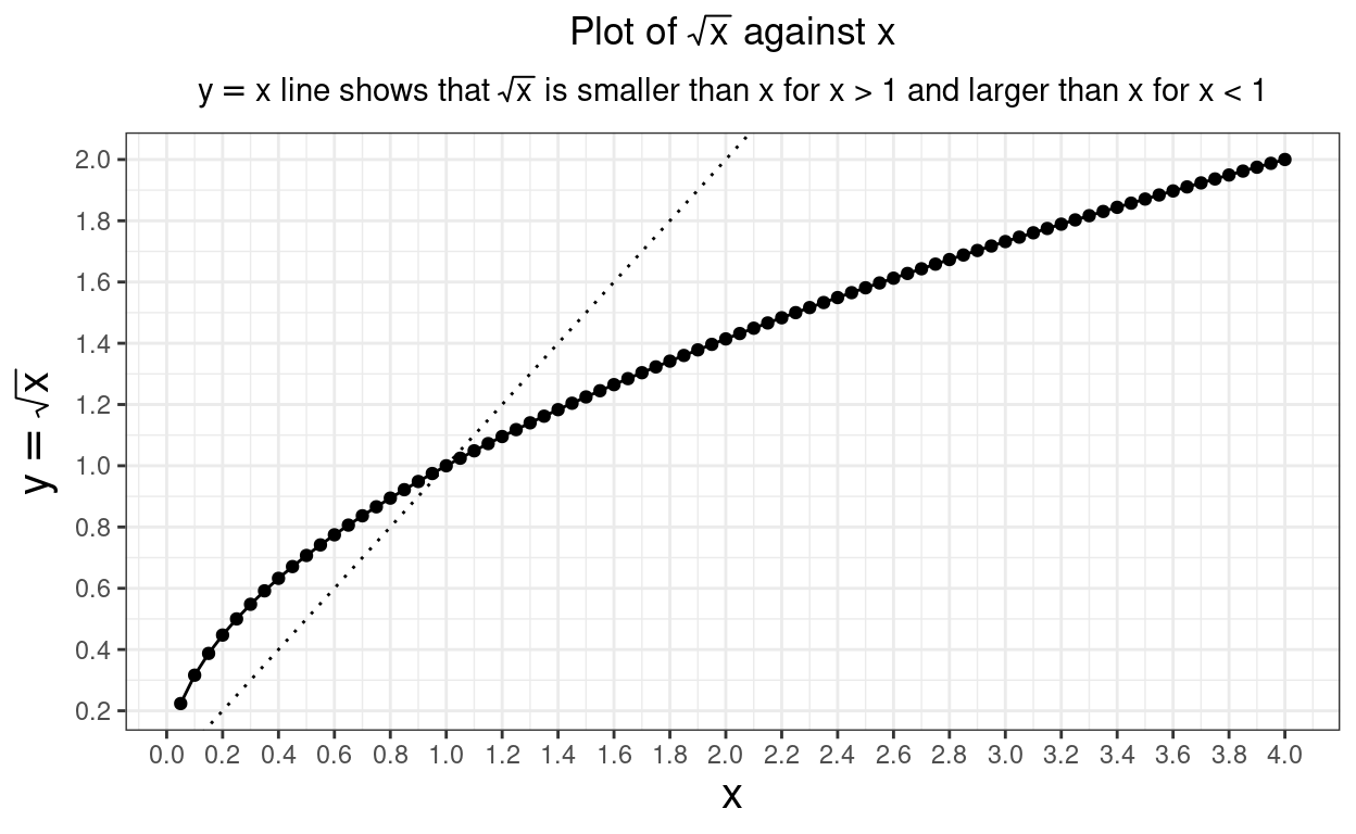
Show code
# ggsave(filename = "transform_sqrt2.png",
#        width = 2000,
#        height = 2000,
#        units = "px")
Variance glossary entry
Show code
tibble(ID = as.character(1:3),
       x = c(1, 7, 10)) %>%
  mutate(mean = mean(x),
         discrep = x - mean,
         discrepSq = discrep^2) -> tmpTib

tmpTib %>%
  summarise(across(x:discrepSq, mean)) %>%
  mutate(ID = "Mean:") %>%
  select(ID, everything()) -> tmpTibMeans

tmpTib %>%
  summarise(across(x:discrepSq, sum)) %>%
  mutate(ID = "Sum:") %>%
  select(ID, everything()) -> tmpTibSums

tmpTib %>%
  bind_rows(tmpTibSums,
            tmpTibMeans) %>%
  write_csv(file = "variance1.csv")

tmpTib %>%
  mutate(y = 1:3,
         y0 = 0, ymax = 3) -> tmpTib

ggplot(tmpTib,
       aes(x = x)) +
  # geom_linerange(aes(x = x, ymin = y0, ymax = ymax)) +
  geom_point(aes(y = y)) +
  geom_vline(xintercept = 6,
             colour = "blue") +
  geom_segment(aes(x = x, xend = mean, y = y, yend = y),
                 colour = "green",
                 arrow = arrow(length = unit(.15, "inches"),
                               ends = "both")) +
  ylim(0.5, 3.5) +
  scale_x_continuous(breaks = 0:12,
                     limits = c(0, 12)) +
  theme(axis.ticks.y = element_blank(),
        axis.text.y = element_blank(),
        axis.title.y = element_blank(),
        panel.grid.major.y = element_blank(),
        panel.grid.minor.y = element_blank()) +
  ggtitle("Discrepancies between observations and the mean",
          subtitle = "Observations are black points, their mean is the blue reference line")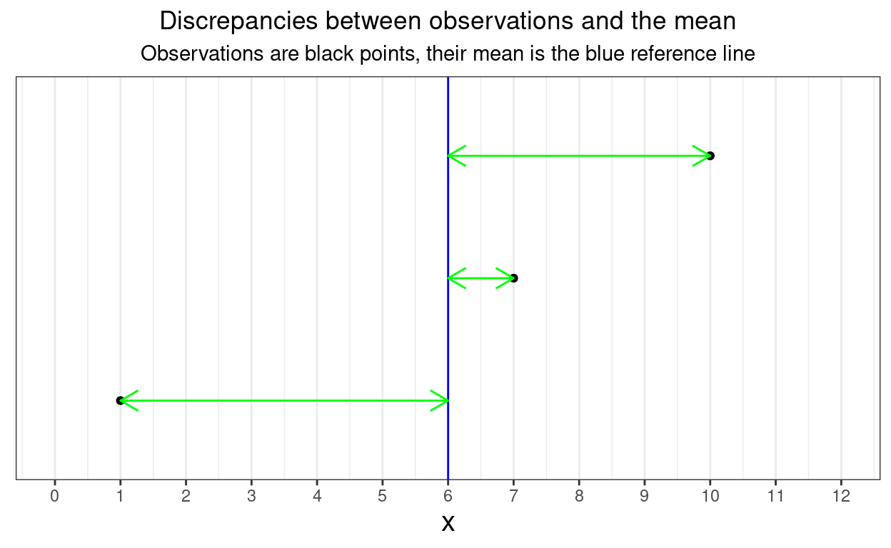
Show code
ggsave(filename = "discrepancies.png",
       width = 2000,
       height = 2000,
       units = "px")
Show code
tibble(n = 3:50) %>%
  mutate(meanDiscrepSq = 5,
       estPopVar = meanDiscrepSq * n / (n - 1)) -> tmpTib

ggplot(data = tmpTib,
       aes(x = n, y = estPopVar)) +
  geom_point() +
  geom_hline(yintercept = 5,
             colour = "blue") +
  ylab("Variance") +
  ylim(c(0, 8)) +
  ggtitle("Plot of estimated population variance for observed variance in sample of 5",
          subtitle = "Blue line shows observed variance")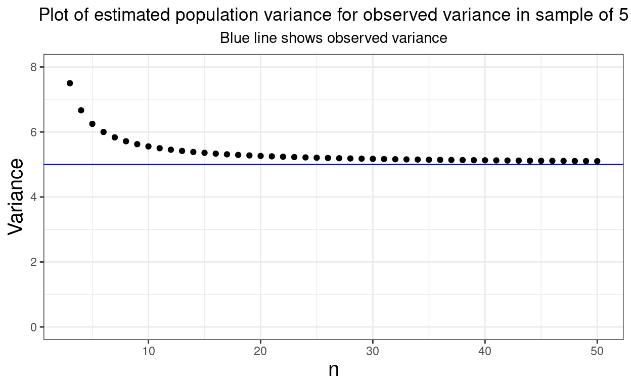
Show code
ggsave(filename = "varianceBias1.png",
       width = 2000,
       height = 2000,
       units = "px")
Now a simulation.
Show code
tibble(n = c(3:10, seq(15, 50, 5))) %>%
  mutate(rep = list(1:1000)) %>%
  unnest_longer(rep) %>%
  rowwise() %>%
  mutate(sample = list(rnorm(n, sd = sqrt(5))),
         varEst = var(sample),
         varObs = varEst * (n - 1) / n) %>%
  ungroup() %>%
  select(-sample) -> tmpTib

tmpTib %>%
  group_by(n) %>%
  summarise(meanVarEst = mean(varEst),
         meanVarObs = mean(varObs)) -> tmpTibMeans

ggplot(data = tmpTib,
       aes(x = n)) +
  geom_violin(aes(y = varObs, group = n),
              fill = "grey") +
  geom_point(data = tmpTibMeans,
             aes(x = n, y = meanVarObs)) +
  geom_hline(yintercept = 5,
             colour = "blue") +
  ylab("Estimated population variance") +
  xlab("Sample size (n)") +
  ggtitle("Observed variances i.e. denominator n, against sample size",
          subtitle = paste0("Violin plot shapes show actual values from n = 1,000 simulations",
                            "\nDots mark mean values per sample size, blue line is true population variance, 5"))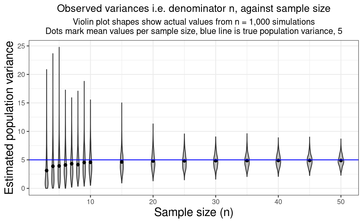
Show code
# ggsave(filename = "varianceBias2.png",
#        width = 2000,
#        height = 2000,
#        units = "px")
That clearly shows the bias: underestimating variance and that it decreases with sample size.
Show code
ggplot(data = tmpTib,
       aes(x = n)) +
  geom_violin(aes(y = varEst, group = n),
              fill = "grey") +
  geom_point(data = tmpTibMeans,
             aes(x = n, y = meanVarEst)) +
  geom_hline(yintercept = 5,
             colour = "blue") +
  ylab("Estimated population variance") +
  xlab("Sample size (n)") +
  ggtitle("Plot of estimated variances against sample size",
          subtitle = paste0("Violin plot shapes show actual values from n = 1,000 simulations",
                            "\nDots mark mean values per sample size, blue line is true population variance, 5"))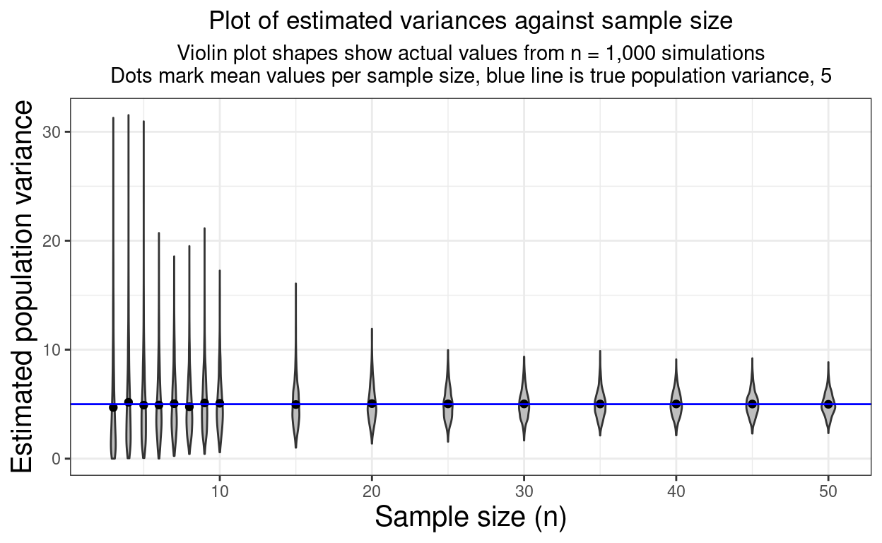
Show code
# ggsave(filename = "varianceBias3.png",
#        width = 2000,
#        height = 2000,
#        units = "px")
That shows that using the denominator of n - 1 corrects the bias and estimates the population variance (set at 5) without bias.
Linear regression
Very simple stuff for the linear regression entry.
Show code
tibble(x = seq(-1, 4, .02)) %>%
  mutate(y = .5 * x + 1) -> tmpTib

ggplot(data = tmpTib,
       aes(x = x, y = y)) +
  geom_line(linewidth = 2) +
  geom_vline(xintercept = 0,
             linetype = 1) +
  geom_hline(yintercept = 0,
             linetype = 1) +
  annotate("text",
           x = .1, y = 2.2,
           parse = TRUE,
           label = "y == .5 * x + 1",
           hjust = 0,
           size = 10) +
  ggtitle("Illustration of simple linear regression line") +
  theme(plot.title = element_text(size = 24),
        plot.subtitle = element_text(size = 18))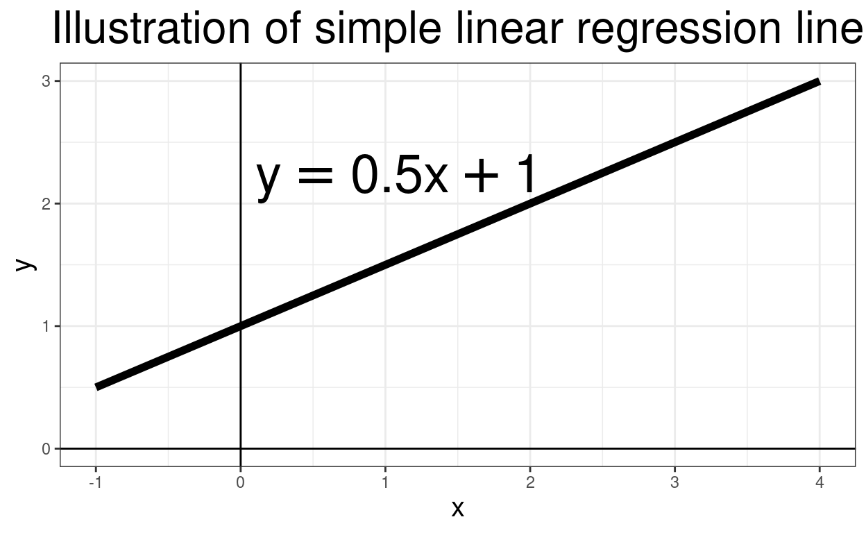
Show code
# ggsave(filename = "linearRegression1.png",
#        width = 3000,
#        height = 2000,
#        units = "px")
Label the intercept
Show code
tibble(x = 0,
       y = 1) -> tmpTibIntercept

ggplot(data = tmpTib,
       aes(x = x, y = y)) +
  geom_line(linewidth = 2) +
  geom_vline(xintercept = 0,
             linetype = 1) +
  geom_hline(yintercept = 0,
             linetype = 1) +
  geom_point(data = tmpTibIntercept,
             size = 5) +
  geom_hline(yintercept = 1,
             linetype = 3) +
  annotate("text",
           x = .1, y = 2.2,
           parse = TRUE,
           label = "y == .5 * x + 1",
           hjust = 0,
           size = 10) +
  ggtitle("Illustration of simple linear regression line",
          subtitle = "Intercept point labelled with reference line") +
  theme(plot.title = element_text(size = 24),
        plot.subtitle = element_text(size = 18))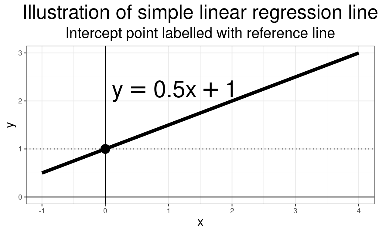
Show code
# ggsave(filename = "linearRegression2intercept.png",
#        width = 3000,
#        height = 2000,
#        units = "px")
Explain the slope
Show code
ggplot(data = tmpTib,
       aes(x = x, y = y)) +
  geom_line(linewidth = 1) +
  geom_vline(xintercept = 0,
             linetype = 1) +
  geom_hline(yintercept = 0,
             linetype = 1) +
  geom_point(data = tmpTibIntercept,
             size = 5) +
  geom_hline(yintercept = 1,
             linetype = 3) +
  geom_segment(aes(x = 2, xend = 3, y = 2, yend = 2),
                 arrow = arrow(ends = "last",
                               angle = 12,
                               length = unit(5, "mm"),
                               type = "closed")) +
  geom_segment(aes(x = 3, xend = 3, y = 2, yend = 2.5),
                 arrow = arrow(ends = "last",
                               angle = 12,
                               length = unit(5, "mm"),
                               type = "closed")) +
  annotate("text",
           x = 2.5, y = 1.9,
           label = "1",
           hjust = .5,
           size = 5) +
  annotate("text",
           x = 3.13, y = 2.25,
           label = "0.5",
           hjust = .5,
           size = 5) +
  annotate("text",
           x = .1, y = 2.2,
           parse = TRUE,
           label = "y == .5 * x + 1",
           hjust = 0,
           size = 10) +
    ggtitle("Illustration of simple linear regression line",
          subtitle = "Slope explained") +
  theme(plot.title = element_text(size = 24),
        plot.subtitle = element_text(size = 18))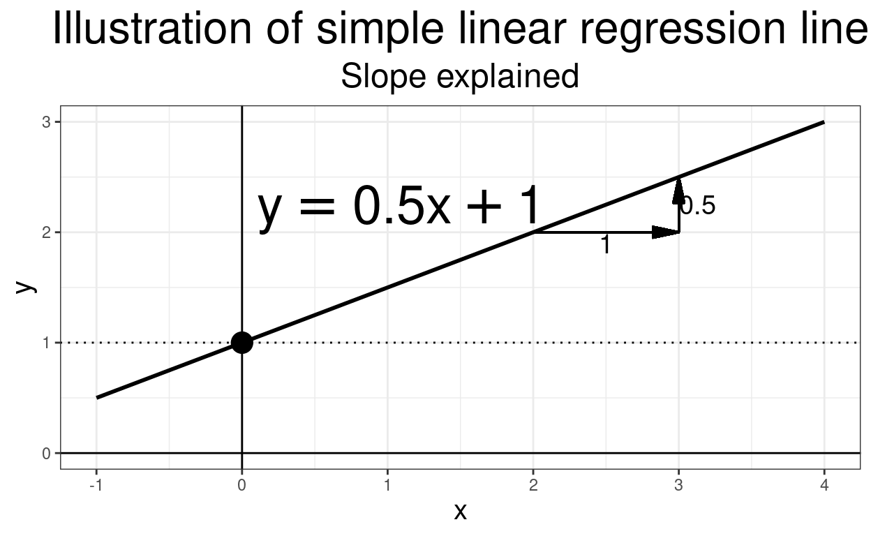
Show code
# ggsave(filename = "linearRegression3slope.png",
#        width = 3000,
#        height = 2000,
#        units = "px")
Add noise. (I confess I tinkered with the seed to get what I wanted!)
Show code
set.seed(1)
nrow(tmpTib) -> n

tmpTib %>%
  mutate(y2 = y + rnorm(n, mean = 0, sd = .25)) -> tmpTib2

ggplot(data = tmpTib2,
       aes(x = x, y = y2)) +
  geom_line(aes(y = y)) +
  geom_point(alpha = .5) +
  geom_smooth(method = "lm") +
  geom_vline(xintercept = 0,
             linetype = 1) +
  geom_hline(yintercept = 0,
             linetype = 1) +
  annotate("text",
           x = .1, y = 2.2,
           parse = TRUE,
           label = "y == .5 * x + 1",
           hjust = 0,
           size = 10) +
  ggtitle("Illustration of simple linear regression line",
          subtitle = "With random Gaussian noise added") +
  theme(plot.title = element_text(size = 24),
        plot.subtitle = element_text(size = 18))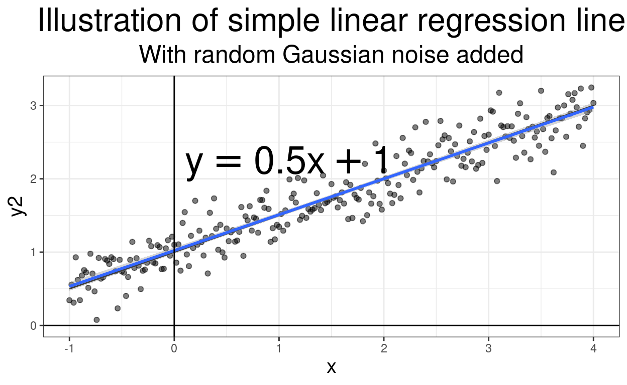
Show code
# ggsave(filename = "linearRegression1noisy.png",
#        width = 3000,
#        height = 2000,
#        units = "px")

### get the lm
lm(tmpTib2$y2 ~ tmpTib2$x) -> tmpLm
The intercept of that best fit linear regression is 1.022 and the slope is 0.489.
Attenuation
This was just to create a plot and table for a glossary entry about attenuation by unreliability of measurement.
Show code
set.seed(12345)
n <-5000 # the number of points per simulation
nNoise <- 6 # the number of levels of noise I am going to inject
matCorr <- matrix(c(1, .9, .9, 1), nrow = 2) # correlation matrix I want (pass it into MASS::mvrnorm())
vecMean <- c(0, 0) # mean vector also needed for MASS::mvrnorm()


as_tibble(MASS::mvrnorm(n = n * nNoise, mu = vecMean, Sigma = matCorr), # does the simulation of the samples
          ### need this to stop as_tibble() grumbling
          .name_repair = "unique") %>%
  ### but I want better variable names so ...
  rename(xpopn = `...1`,
         ypopn = `...2`) %>%
  ### now create a long variable of the levels of noise to add
  mutate(noise = rep(seq(0, 1, .2), each = n)) %>%
  ### now use those noise values to add the noise!
  rowwise() %>%
  mutate(x = xpopn + rnorm(1, sd = noise),
         y = ypopn + rnorm(1, sd = noise)) %>%
  ungroup() -> tmpTib

### plot that (I never got a plot I really liked but it will do)
ggplot(data = tmpTib,
       aes(x = x, y = y)) +
  facet_wrap(facets = vars(noise),
             ncol = 2) +
  geom_smooth(method = "lm") +
  geom_point(alpha = .05) +
  ### for Rblog
  ggpubr::stat_cor(size = 3, label.y = 4.2) +
  ggpubr::stat_regline_equation(size = 3, label.y = 2.5) +
  ### to save for the glossary
  # ggpubr::stat_cor(size = 5, label.y = 4.2) +
  # ggpubr::stat_regline_equation(size = 5, label.y = 2.5)
 theme_bw()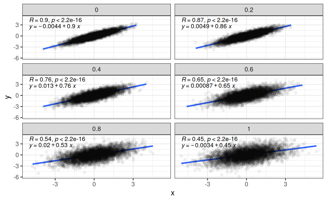
Show code
# ggsave(filename = "attenuation.png",
#        height = 2400,
#        width = 3200,
#        units = "px")
I think that shows clearly enough the impact of the added noise attenuating the correlation and reducing the slope
Show code
tmpTib %>%
  group_by(noise) %>%
  summarise(sampCorr = cor(x, y)) %>%
  mutate(rel = 1 / (1 + noise^2),
         attCorrectedCorr = sampCorr / rel) -> tmpTibSummary

tmpTibSummary %>%
  select(noise, rel, sampCorr, attCorrectedCorr) %>%
  flextable() %>%
  colformat_double(digits = 3)
noise | rel | sampCorr | attCorrectedCorr |
|---|---|---|---|
0.000 | 1.000 | 0.903 | 0.903 |
0.200 | 0.962 | 0.867 | 0.902 |
0.400 | 0.862 | 0.764 | 0.886 |
0.600 | 0.735 | 0.654 | 0.889 |
0.800 | 0.610 | 0.543 | 0.891 |
1.000 | 0.500 | 0.453 | 0.907 |
Show code
tmpTibSummary %>%
  mutate(across(everything(), ~ sprintf("%05.3f", .x))) %>%
  write_csv(file = "attenuation.csv")
And that showed that the correction:
\[correctedCorr = \frac{corr}{\sqrt{rel_{x}rel_{y}}}\]
works!
Mokken scaling
This was to illustrate the entry on Mokken scaling.
Mokken double monotonicity model
Show code
set.seed(12345)
n <- 500000


irt_p <- function(theta, a, b, c){   #ability and item parameters as scalars
  p <- c + (1 - c) / (1 + exp(-1.7 * a * (theta - b)))

  p
}

tibble(theta = seq(-4, 4, .1)) %>%
  mutate(Item1 = irt_p(theta, a = 1, b = -1, c = 0),
         Item2 = irt_p(theta, a = 1, b = 1, c = 0)) %>%
  pivot_longer(cols = c(Item1, Item2),
               names_to = "Item",
               values_to = "p")-> tmpTib

ggplot(data = tmpTib,
       aes(x = theta, y = p, colour = Item)) +
  # geom_point() +
  geom_line(linewidth = 2) +
  ylab("Probability of answering 'yes' to item") +
  xlab("Person's true value on the latent variable") +
  ggtitle("Two item response curves, Mokken double monotonicity model",
subtitle = "Reponse curves have same shape and don't cross") 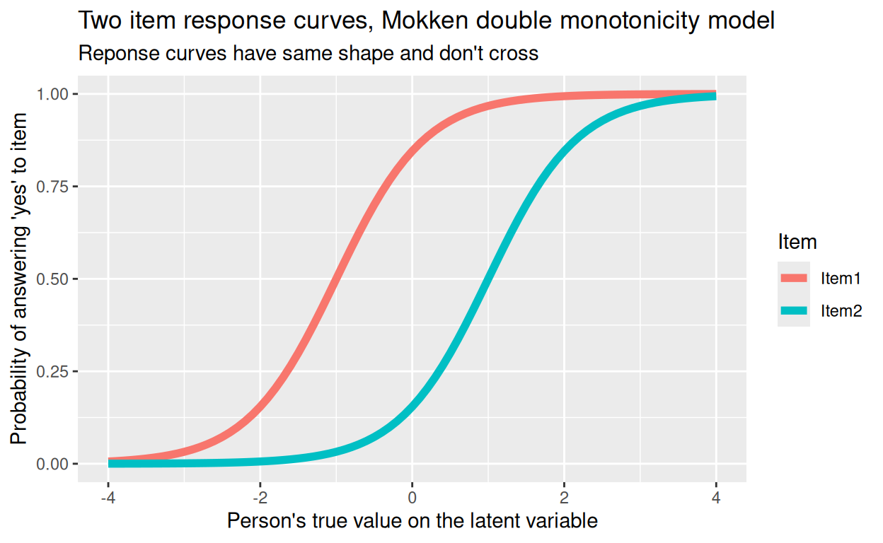
Mokken monotone homogeneity model
Show code
tibble(theta = seq(-8, 8, .1)) %>%
  mutate(Item1 = irt_p(theta, a = 1, b = -1, c = 0),
         Item2 = irt_p(theta, a = .3, b = .1, c = 0)) %>%
  pivot_longer(cols = c(Item1, Item2),
               names_to = "Item",
               values_to = "p")-> tmpTib

ggplot(data = tmpTib,
       aes(x = theta, y = p, colour = Item)) +
  # geom_point() +
  geom_line(linewidth = 2) +
  ylab("Probability of answering 'yes' to item") +
  xlab("Person's true value on the latent variable") +
  ggtitle("Two item response curves, Mokken monotone homogeneity model",
subtitle = "Reponse curves still monotone but can differ in slope and can cross") 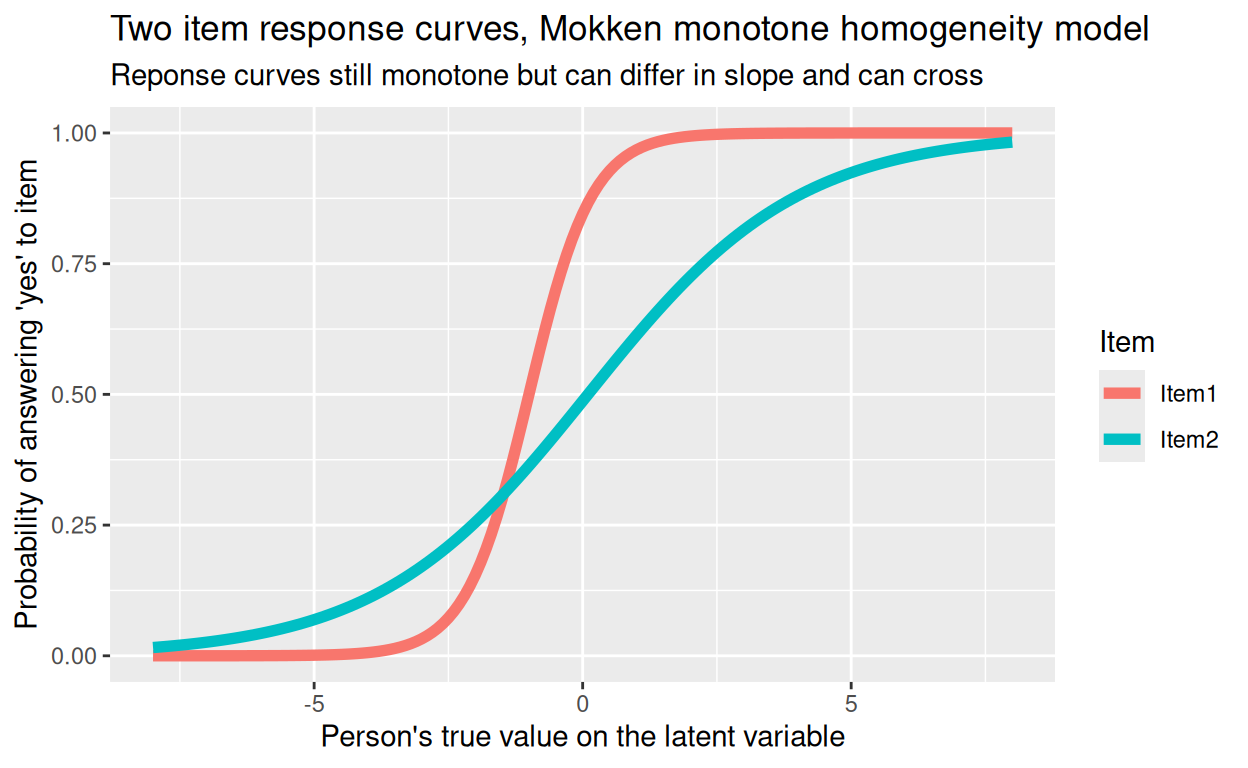
IRT (Item Response Theory)
This, leaning heavily on the above code for the Mokken scaling entry, was to give basics of IRT.
One parameter model
Show code
tibble(theta = seq(-4, 4, .1)) %>%
  mutate(Item1 = irt_p(theta, a = 1, b = -1, c = 0),
         Item2 = irt_p(theta, a = 1, b = 1, c = 0)) %>%
  pivot_longer(cols = c(Item1, Item2),
               names_to = "Item",
               values_to = "p")-> tmpTib

tmpTib %>%
  mutate(delta = abs(p - .5)) %>%
  group_by(Item) %>%
  mutate(minDelta = abs(min(delta))) %>%
  filter(delta == minDelta) -> tibLocations

ggplot(data = tmpTib,
       aes(x = theta, y = p, colour = Item)) +
  geom_line(linewidth = 2) +
  geom_hline(yintercept = .5,
             linetype = 3) +
  geom_vline(data = tibLocations,
             aes(xintercept = theta,
                 colour = Item),
             linetype = 1) +
  ylab("Probability of answering 'yes' to item") +
  xlab("Person's true value on the latent variable") +
  ggtitle("Two item response curves, one parameter IRT model",
subtitle = "Reponse curves have same shape but different locations shown by vertical reference lines") 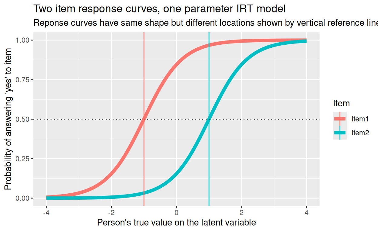
Two parameter model
Show code
tibble(theta = seq(-8, 8, .1)) %>%
  mutate(Item1 = irt_p(theta, a = 1, b = -1, c = 0),
         Item2 = irt_p(theta, a = .3, b = .1, c = 0)) %>%
  pivot_longer(cols = c(Item1, Item2),
               names_to = "Item",
               values_to = "p")-> tmpTib

tmpTib %>%
  mutate(delta = abs(p - .5)) %>%
  group_by(Item) %>%
  mutate(minDelta = abs(min(delta))) %>%
  filter(delta == minDelta) -> tibLocations

ggplot(data = tmpTib,
       aes(x = theta, y = p, colour = Item)) +
  geom_line(linewidth = 2) +
  geom_hline(yintercept = .5,
             linetype = 3) +
  geom_vline(data = tibLocations,
             aes(xintercept = theta,
                 colour = Item),
             linetype = 1) +
  ylab("Probability of answering 'yes' to item") +
  xlab("Person's true value on the latent variable") +
  ggtitle("Two item response curves, two parameter IRT model",
subtitle = "Reponse curves still monotone but different locations shown by vertical reference lines\nand different slopes") 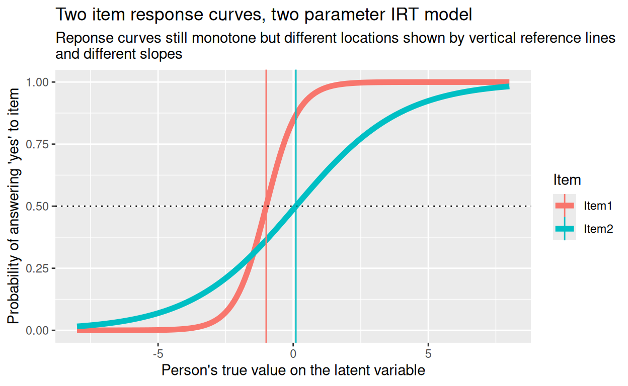
Three parameter model
Show code
tibble(theta = seq(-8, 8, .1)) %>%
  mutate(Item1 = irt_p(theta, a = 1, b = -1, c = 0),
         Item2 = irt_p(theta, a = .3, b = .1, c = 0.25)) %>%
  pivot_longer(cols = c(Item1, Item2),
               names_to = "Item",
               values_to = "p")-> tmpTib

ggplot(data = tmpTib,
       aes(x = theta, y = p, colour = Item)) +
  geom_line(linewidth = 2) +
  geom_line(linewidth = 2) +
  geom_hline(yintercept = .5,
             linetype = 3) +
  ylab("Probability of answering 'yes' to item") +
  xlab("Person's true value on the latent variable") +
  ggtitle("Two item response curves, three parameter IRT model",
          subtitle = "Reponse curves differ in location, slope and 'guessing' rate") +
  labs(caption = "Item2 has .25 guessing rate, Item1 has zero guessing rate ") +
  theme(plot.caption = element_text(hjust = .5))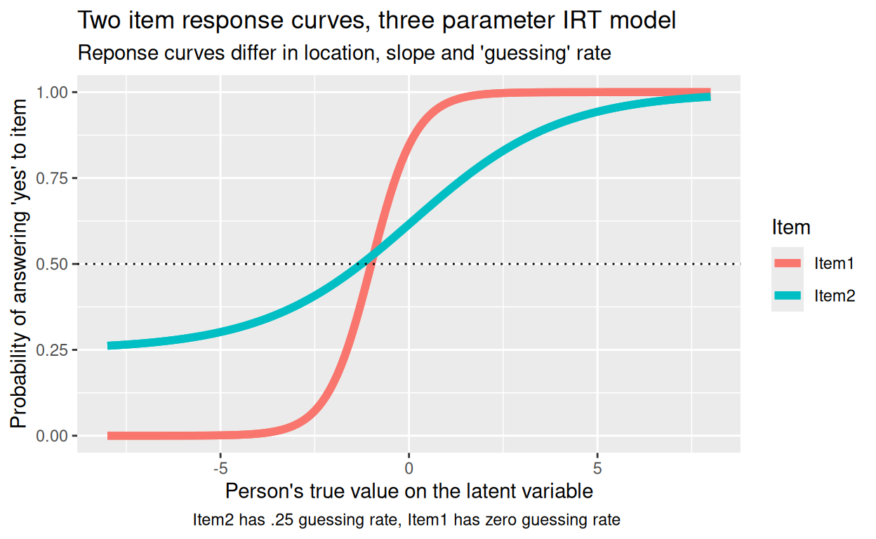
The Rasch model
Show code
library(tidyverse)

### set ggplot theme defaults
theme_set(theme_bw())
theme_update(plot.title = element_text(hjust = .5),
             plot.subtitle = element_text(hjust = .5))

funRasch <- function(p, i){
  ### this is basically the logistic function
  diff <- p - i
  pr <- exp(diff) / (1 + exp(diff))
}

n <- 5000 # to get nice smooth lines

tibble(person = seq(-5, 8, length.out = n)) %>% # sets range of person locations
  ### and now create probabilities per person for two items
  mutate(Item_1 = funRasch(person, 1),
         Item_2 = funRasch(person, 2)) -> tmpTib

### pivot longer to make nice plot easier
tmpTib %>%
  pivot_longer(cols = -person,
               names_to = "Item",
               values_to = "prob") -> tmpTibLong

### find the locations for each item at which probability
### is nearest to .5
tmpTibLong %>%
  mutate(delta = abs(prob - .5)) %>%
  group_by(Item) %>%
  mutate(minDelta = abs(min(delta))) %>%
  filter(delta == minDelta) -> tibLocations

### plot this
ggplot(data = tmpTibLong,
       aes(x = person,
           y = prob,
           colour = Item)) +
  ### the item response curves
  geom_line(linewidth = 2) +
  ### show the item locations, first the .5 reference line
  geom_hline(yintercept = .5,
             linetype = 3,
             linewidth = 1.5) +
  ### and now the locations
  geom_vline(data = tibLocations,
             aes(xintercept = person,
                 colour = Item),
             linetype = 2,
             linewidth = 1.5) +
  ylab("Probability of person answering 'Y' to Item") +
  scale_x_continuous("Person's location on scale of variable to be measured",
                     breaks = -5:8) +
  ggtitle("Probability of answering positively to two perfect Rasch model items",
       subtitle = paste0("Horizontal reference line p = .5",
                         "\nVertical reference lines give locations of the items")) +
  ### increase size of text for the web
  theme(text = element_text(size = 20))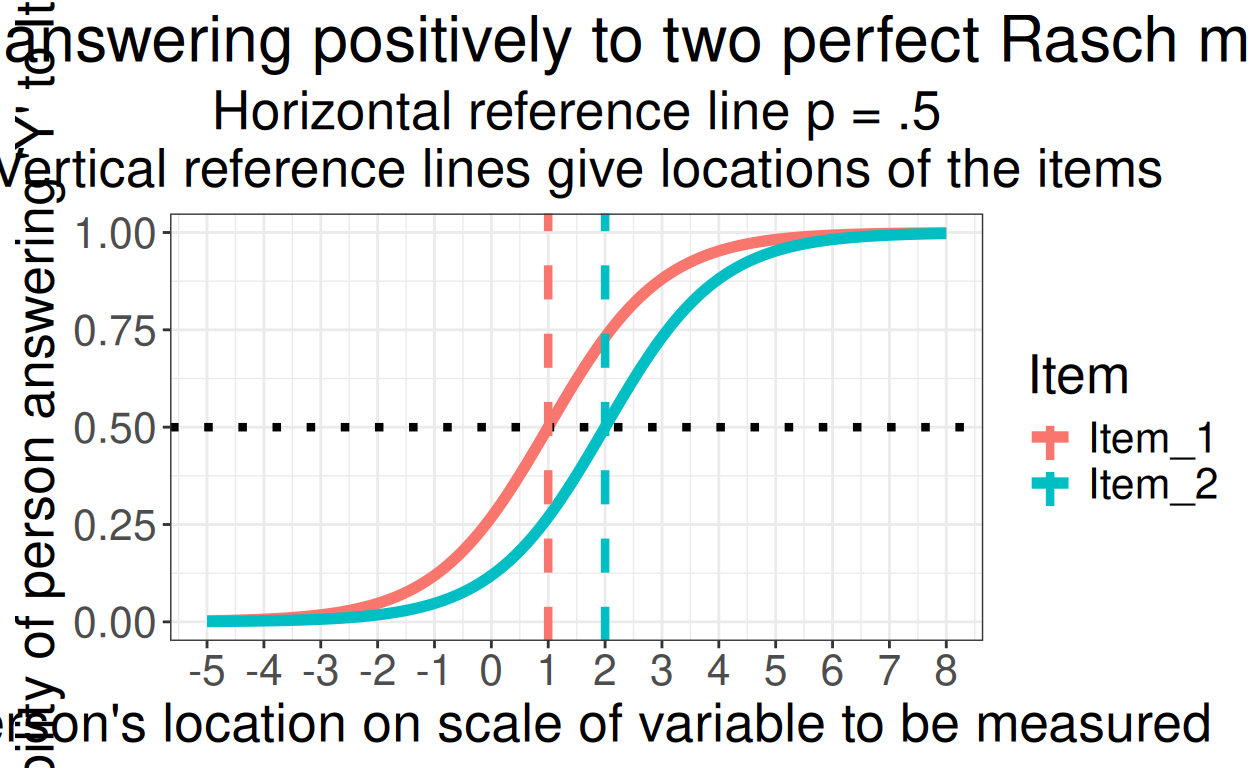
Odds ratios and probabilities
Show code
getOdds <- function(prob) {
  prob / (1 - prob)
  }
getOdds <- Vectorize(getOdds)
tibble(prob = seq(0.001, .999, .005)) %>%
  mutate(odds = getOdds(prob),
         logOdds = log(odds),
         diff = odds - prob) -> tmpTib

tmpTib %>%
  pivot_longer(cols = c(odds, logOdds)) %>%
  mutate(transform = if_else(name == "odds",
                             "raw",
                             "log"),
         refVal = if_else(transform == "raw",
                          1,
                          0)) -> tmpTibLong

ggplot(data = tmpTib,
       aes(x = prob, y = odds)) +
  geom_point(alpha = .2) +
  geom_line() +
  geom_vline(xintercept = .5,
             linetype = 3) +
  geom_hline(yintercept = 1,
             linetype = 3) +
  xlab("Probability") +
  ylab("Odds ratio") +
  ggtitle("Plot of odds ratio against probability")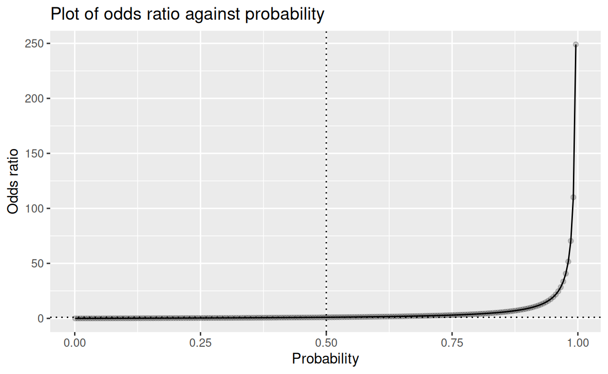
Show code
ggsave(filename = "ods_vs_prob.png",
       width = 1700,
       height = 1470,
       units = "px")
Show code
ggplot(data = tmpTib,
       aes(x = odds, y = prob)) +
  geom_point(alpha = .2) +
  geom_line() +
  geom_hline(yintercept = .5,
             linetype = 3) +
  geom_vline(xintercept = 1,
             linetype = 3) +
  xlab("Odds ratio") +
  ylab("Probability") +
  ggtitle("Plot of probability against odds ratio")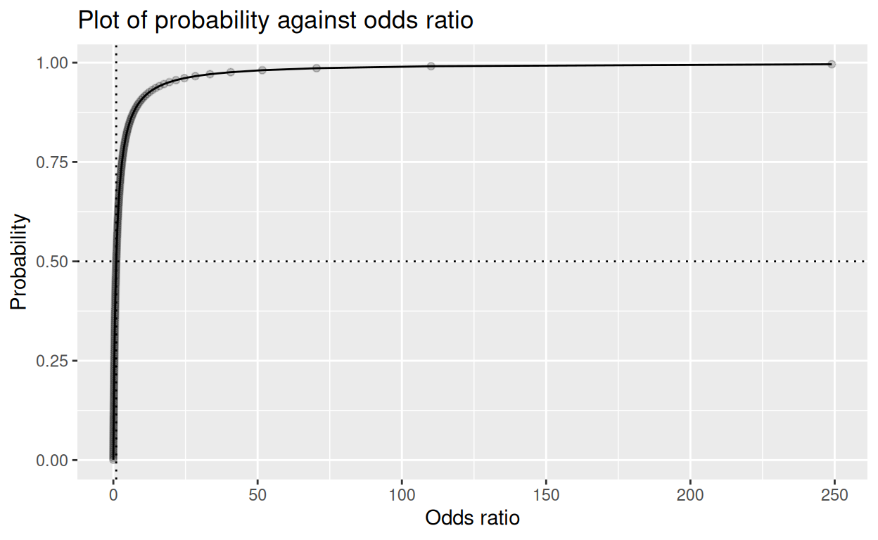
Show code
ggsave(filename = "prob_vs_odds.png",
       width = 1700,
       height = 1470,
       units = "px")
Show code
ggplot(data = tmpTibLong,
       aes(x = prob, y = value)) +
  facet_grid(rows = vars(transform),
            scales = "free_y") +
  geom_point(alpha = .2) +
  geom_line() +
  geom_vline(xintercept = .5,
             linetype = 3) +
  geom_hline(aes(yintercept = refVal)) +
  xlab("Probability") +
  ylab("Value (odds ratio or log odds)") +
  ggtitle("Plot of odds ratio and log odds ratio against probability")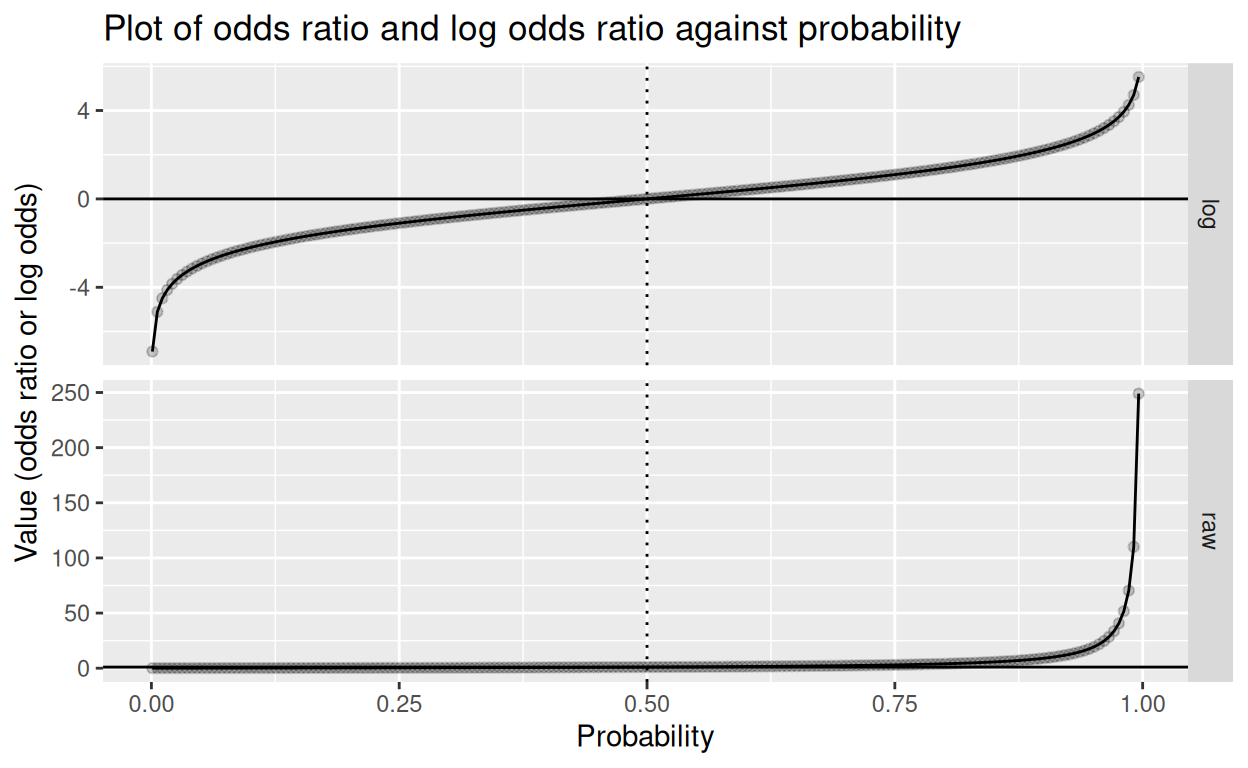
Show code
ggsave(filename = "ods_and_logOdds_vs_prob.png",
       width = 1700,
       height = 1470,
       units = "px")
Show code
save.image(file = "Glossary.rda")

load(file = "Glossary.rda")free counter