Shiny app
There is now a shiny app using this function here.
This post
Until last week (November 2023!) if I wanted a confidence interval (CI) for a Spearman correlation given the n that created it I used an analytic, parametric method which is actually for the Pearson correlation and I think I was not alone in doing that. However, I have just discovered that there are better approaches and that work on them goes back to the mid 20th Century. Ooops.
They are all approximations that drew on parametric models and if you have raw data, you are far better off using a bootstrap method to get your CI. However, if you are looking at a Spearman correlation in the literature and only have that and the n then you can get a CI but you seem to have a choice of four ways of doing this.
So here are the 95% CIs for observed correlations of zero, .5 and .8 for n from 8 to 100.
Show code
tibble(n = list(8:100), rs = list(.8, .5, 0)) %>%
  unnest_longer(rs) %>%
  unnest_longer(n) %>%
  rowwise() %>%
  mutate(CIGBW = list(getCISpearman(rs, n, Gaussian = TRUE, FHP = FALSE)),
         CItBW = list(getCISpearman(rs, n, Gaussian = FALSE, FHP = FALSE)),
         CIGFieller = list(getCISpearman(rs, n, Gaussian = TRUE, FHP = TRUE)),
         CItFieller = list(getCISpearman(rs, n, Gaussian = FALSE, FHP = TRUE))) %>%
  ungroup() %>%
  unnest_longer(col = starts_with("CI"), simplify = FALSE) %>%
  rename(limit = CIGBW_id) %>%
  select(-ends_with("_id")) %>%
  select(n, rs, limit, everything()) -> tibCLs

# tibCLs %>%
#   mutate(diffGauss = CIGBW - CIGFieller,
#          sqDiffGauss = diffGauss^2,
#          difft = CItBW - CItFieller,
#          sqDifft = difft^2) %>%
#   summarise(across(diffGauss : sqDifft, mean))

tibCLs %>%
  pivot_longer(cols = starts_with("CI")) %>%
  rename(method = name) %>%
  mutate(Method = case_when(
    method == "CIGBW" ~ "B&W, Gaussian",
    method == "CItBW" ~ "B&W, t dist.",
    method == "CIGFieller" ~ "FH&P, Gaussian",
    method == "CItFieller" ~ "FH&P, t dist."),
    approx = if_else(str_detect(Method, fixed("B&W")), "B&W", "FH&P"),
    distribn = if_else(str_detect(Method, fixed("Gaussian")), "Gaussian", "t dist.")) -> tibCLsLong

ggplot(data = tibCLsLong,
       aes(x = n, y = value, colour = method, shape = method))  +
  facet_grid(rows = vars(rs)) +
  geom_point(size = .4) +
  geom_hline(aes(yintercept = rs)) +
  ylim(c(-1, 1))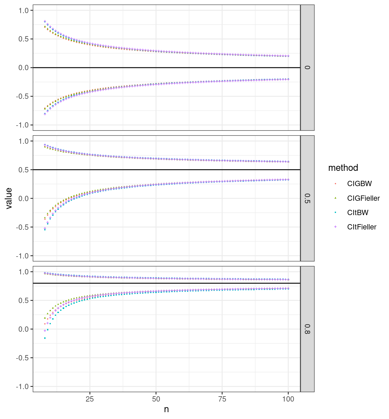
That illustrates several things:
Of course the CI is symmetrical around zero for the null case of no correlation but it is asymmetrical around the observed correlation for non-zero observed correlations, more so the stronger the correlation.
The methods differ in the widths of their CIs more for smaller n and for stronger correlations.
By n = 100 the differences between the methods are negligible.
It looks as if the differences between the methods are consistent across the values for n within each observed correlation and confidence limit (i.e. LCL or UCL) but it’s hard to eyeball that from the plot.
So here is the same plot but just for n from 8 to 15.
Show code
tibCLsLong %>%
  filter(n <= 15) -> tmpTib

ggplot(data = tmpTib,
       aes(x = n, y = value, colour = method, shape = method))  +
  facet_grid(rows = vars(rs)) +
  geom_point(size = .4) +
  geom_hline(aes(yintercept = rs)) +
  ylim(c(-.85, 1))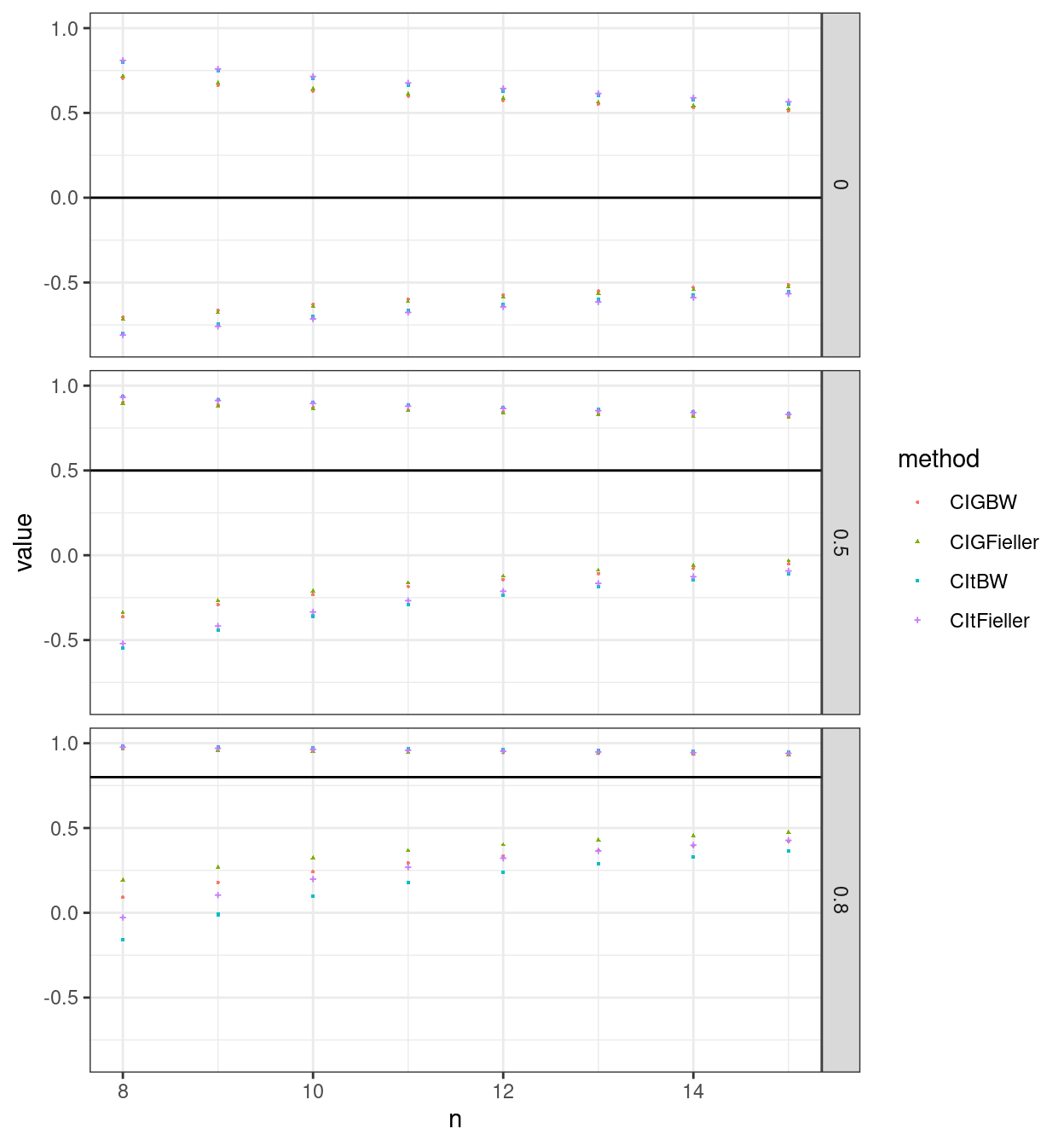
The four methods involve two different changes: the approximation to the standard error of the correlation and whether to look that up against the Gaussian distribution or against the t distribution with df = n - 2. The next two plots facet the issues in the two possible different orders.
This first plot pulls the issue of looking up against the Gaussian or t distributions to the columns in the facetted plot allowing a clearer comparison of the two approximations to the SE of the correlation.
Show code
ggplot(data = tibCLsLong,
       aes(x = n, y = value, colour = approx))  +
  facet_grid(rows = vars(rs),
             cols = vars(distribn)) +
  geom_point(size = .4) +
  geom_hline(aes(yintercept = rs)) +
  ylim(c(-1, 1))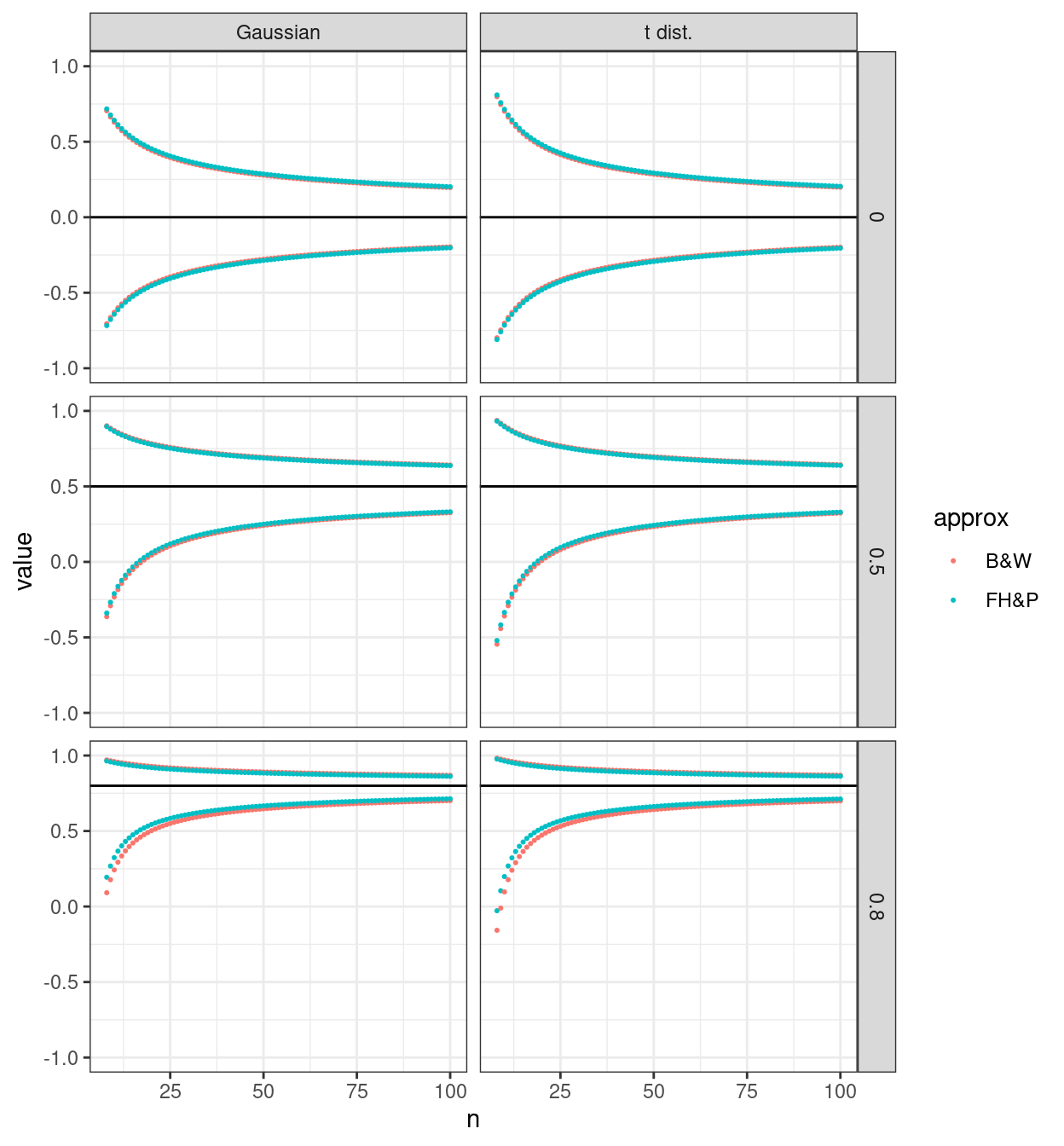
That seems to show fairly clearly that for the zero correlation case the B&W, i.e. the Bonett & White (2000) approximation gives slightly tighter CIs than the FH&P, i.e. the Fieller, Hartley & Pearson (1957) one but that the approximations have the reverse relationship with CI widths for the non-zero correlations.
This next plot makes it easy to look at how the choice of lookup, against the Gaussian or the t distributions affects the CIs.
Show code
ggplot(data = tibCLsLong,
       aes(x = n, y = value, colour = distribn))  +
  facet_grid(rows = vars(rs),
             cols = vars(approx)) +
  geom_point(size = .4) +
  geom_hline(aes(yintercept = rs)) +
  ylim(c(-1, 1))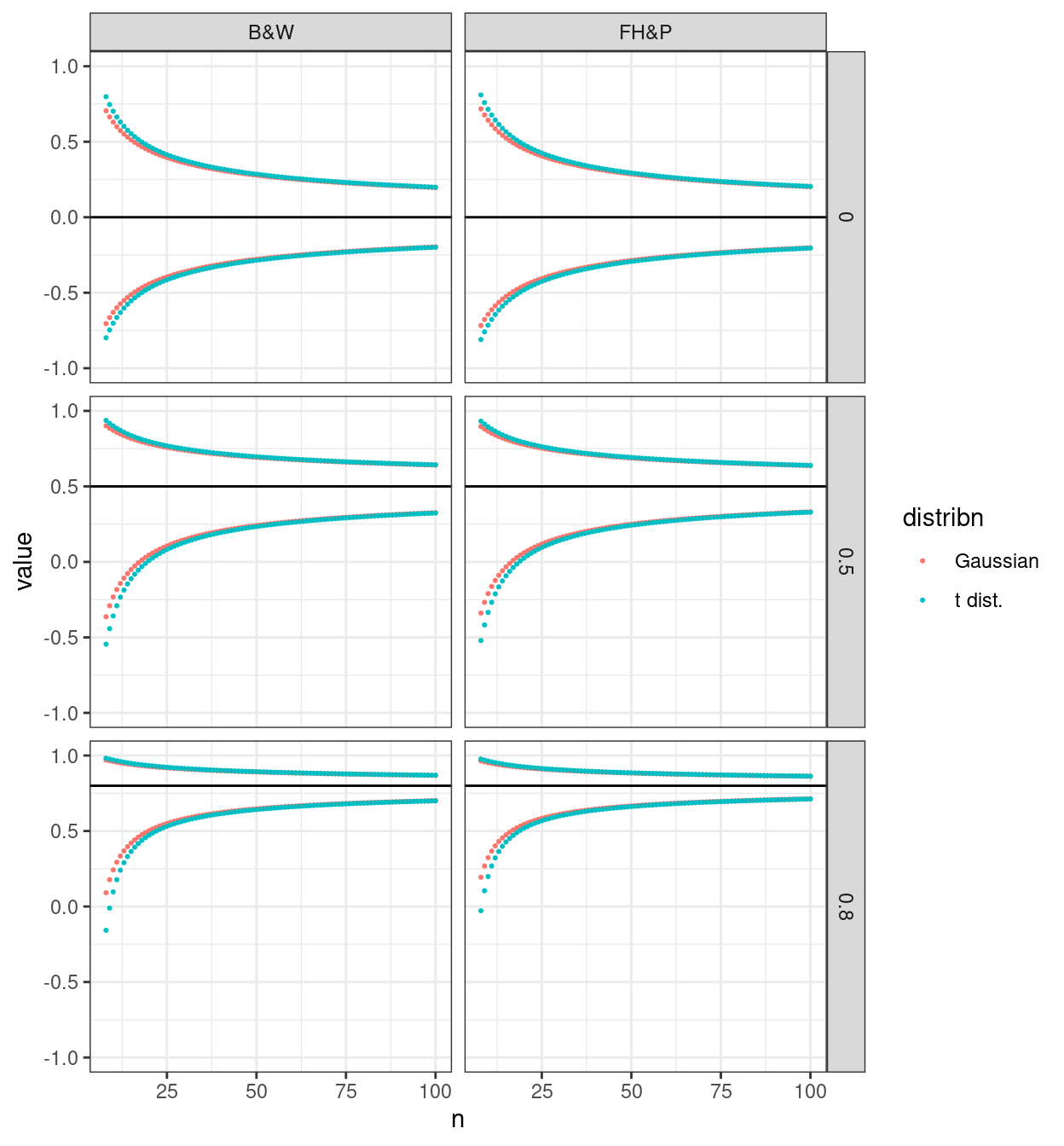
So the Gaussian method gives tighter CIs. However, simulation work I think suggests that these are slightly too tight and that the t distribution method gives coverage closer to 95% in simulations.
Summary
The
getCISpearman()function from the CECPfuns package gives you the four methods of getting a CI around an observed Spearman correlation coefficient.I have set the default to
getCISpearman(rs, n, ci = .95, Gaussian = FALSE, FHP = FALSE)which gets you the Bonett & White (2000) approximation to the SE of the Spearman correlation rather than the Fieller, Hartley & Pearson (1957) method and gets the coverage by looking up the desired coverage (default .95, i.e. 95%) against the t distribution rather than the Gaussian.However, the differences between any of the four possible methods depend on the observed correlation and are trivial for any sensible therapy/MH data and questions for n >= 25 and the methods are known to be very approximate for n < 25.
I haven’t explored this here but the methods known to have poor coverage accuracy as the absolute population correlation goes above .95 so it’s wise to interpret CIs very cautiously for observed correlations above .9.
However, there is evidence from simulations that Pearson correlation CIs are highly sensitive to deviations from bivariate Gaussian population distributions so when data are either clearly not Gaussian or where linear measurement is probably not present, use of these CI estimates for rank correlation methods like the Spearman correlation may be more robust than simple parametric CIs for the Pearson correlation.
However (again!) if you have raw data then bca (“bias correction and acceleration”) bootstrap estimation of a CI around either the observed Pearson or Spearman correlation (depending on your interests and belief about linearity of measurement) will be more robust than these CI estimates that only use the observed correlation and n.
Geeky stuff
This compares the ordering of the CLs from the four methods. It’s pretty geeky as realistically the differences don’t matter for typical therapy/MH work but I have kept this because it interests me and I like the use of order() in the code, but this is angels on the head of a pin stuff!
Show code
rs | n | limit | CItFieller | CItBW | CIGFieller | CIGBW |
|---|---|---|---|---|---|---|
0.0 | ||||||
8 | LCL | -0.8099 | -0.7984 | -0.7175 | -0.7047 | |
9 | LCL | -0.7590 | -0.7467 | -0.6771 | -0.6641 | |
10 | LCL | -0.7150 | -0.7022 | -0.6427 | -0.6296 | |
0.5 | ||||||
8 | LCL | -0.5207 | -0.5451 | -0.3391 | -0.3630 | |
9 | LCL | -0.4174 | -0.4419 | -0.2678 | -0.2907 | |
10 | LCL | -0.3346 | -0.3585 | -0.2102 | -0.2321 | |
0.8 | ||||||
8 | LCL | -0.0280 | -0.1573 | 0.1937 | 0.0913 | |
9 | LCL | 0.1043 | -0.0105 | 0.2681 | 0.1774 | |
10 | LCL | 0.1986 | 0.0969 | 0.3238 | 0.2426 |
That shows that the ordering of the lower CLs is not consistent across observed correlations even for that limited range of n. Here’s the same for the UCL.
Show code
rs | n | limit | CItFieller | CItBW | CIGFieller | CIGBW |
|---|---|---|---|---|---|---|
0.0 | ||||||
8 | UCL | 0.8099 | 0.7984 | 0.7175 | 0.7047 | |
9 | UCL | 0.7590 | 0.7467 | 0.6771 | 0.6641 | |
10 | UCL | 0.7150 | 0.7022 | 0.6427 | 0.6296 | |
0.5 | ||||||
8 | UCL | 0.9323 | 0.9366 | 0.8960 | 0.9013 | |
9 | UCL | 0.9127 | 0.9175 | 0.8794 | 0.8849 | |
10 | UCL | 0.8950 | 0.9003 | 0.8648 | 0.8705 | |
0.8 | ||||||
8 | UCL | 0.9769 | 0.9822 | 0.9641 | 0.9708 | |
9 | UCL | 0.9700 | 0.9761 | 0.9581 | 0.9653 | |
10 | UCL | 0.9637 | 0.9705 | 0.9528 | 0.9603 |
Just to confirm that I turned those limits into rank order across the four methods as shown here for the LCLs and n from 8 to 15.
Show code
tibCLsLong %>%
  filter(limit == "LCL") %>%
  filter(n < 16) %>%
  group_by(rs, n) %>%
  mutate(order = order(value)) %>%
  ungroup() %>%
  select(-c(value, Method, approx, distribn)) %>%
  # mutate(rowN = row_number()) %>%
  pivot_wider(names_from = "method", values_from = "order") %>%
  mutate(rs = sprintf("%3.1f", rs)) %>%
  as_grouped_data(groups = "rs") %>%
  flextable()
rs | n | limit | CIGBW | CItBW | CIGFieller | CItFieller |
|---|---|---|---|---|---|---|
0.8 | ||||||
8 | LCL | 2 | 4 | 1 | 3 | |
9 | LCL | 2 | 4 | 1 | 3 | |
10 | LCL | 2 | 4 | 1 | 3 | |
11 | LCL | 2 | 4 | 1 | 3 | |
12 | LCL | 2 | 4 | 1 | 3 | |
13 | LCL | 2 | 4 | 1 | 3 | |
14 | LCL | 2 | 1 | 4 | 3 | |
15 | LCL | 2 | 1 | 4 | 3 | |
0.5 | ||||||
8 | LCL | 2 | 4 | 1 | 3 | |
9 | LCL | 2 | 4 | 1 | 3 | |
10 | LCL | 2 | 4 | 1 | 3 | |
11 | LCL | 2 | 4 | 1 | 3 | |
12 | LCL | 2 | 4 | 1 | 3 | |
13 | LCL | 2 | 4 | 1 | 3 | |
14 | LCL | 2 | 4 | 1 | 3 | |
15 | LCL | 2 | 4 | 1 | 3 | |
0.0 | ||||||
8 | LCL | 4 | 2 | 3 | 1 | |
9 | LCL | 4 | 2 | 3 | 1 | |
10 | LCL | 4 | 2 | 3 | 1 | |
11 | LCL | 4 | 2 | 3 | 1 | |
12 | LCL | 4 | 2 | 3 | 1 | |
13 | LCL | 4 | 2 | 3 | 1 | |
14 | LCL | 4 | 2 | 3 | 1 | |
15 | LCL | 4 | 2 | 3 | 1 |
Some of the differences in the LCL values that led to those orderings may have been tiny but it’s clear that the methods aren’t consistently ordering the LCLs within a given observed correlation nor are the orders the same for the different observed correlations.
Acknowledgements
This started from finding the excellent answers from onestop and retodomax to the question How to calculate a confidence interval for Spearman’s rank correlation? on CrossValidated. As referenced there …
Bishara, A. J., & Hittner, J. B. (2017). Confidence intervals for correlations when data are not normal. Behavior Research Methods, 49(1), 294–309. https://doi.org/10.3758/s13428-016-0702-8 gives extensive simulation work covering much more than these CIs. I checked my code against the results from the R code given in Supplement A to that paper. Then …
Bonett, D. G., & Wright, T. A. (2000). Sample size requirements for estimating pearson, kendall and spearman correlations. Psychometrika, 65(1), 23–28. https://doi.org/10.1007/BF02294183 is a classic (interesting to see how typesetting of equations has improved since 2000!) and …
Ruscio, J. (2008). Constructing Confidence Intervals for Spearman’s Rank Correlation with Ordinal Data: A Simulation Study Comparing Analytic and Bootstrap Methods. Journal of Modern Applied Statistical Methods, 7(2), 416–434. https://doi.org/10.22237/jmasm/1225512360 was another excellent paper on the topic.
Thanks to all those authors.