Show code
### this is just to create a sensible graphic for this post
### otherwise the first huge facetted histogram comes up
library(latex2exp)
### create limits for the plot area
tibble(x = c(0, 0, 1, 1),
       y = c(.2, .3, .3, .2)) -> tibBox
### create equation
valLabel <- TeX("$RCI = 1.96 * SD_{1} * \\sqrt{2} * \\sqrt{1 - reliability}$")
### plot it
ggplot(data = tibBox,
       aes(x = x, y = y)) +
  annotate("text",
           x = 0,
           y = .25,
           label = valLabel,
           parse = TRUE,
           size = 9) +
  coord_cartesian(ylim = c(.2, .3)) +
  ### remove all distractions
  theme_classic() +
  theme(axis.text = element_blank(),
        axis.title = element_blank(),
        axis.line = element_blank(),
        axis.ticks = element_blank())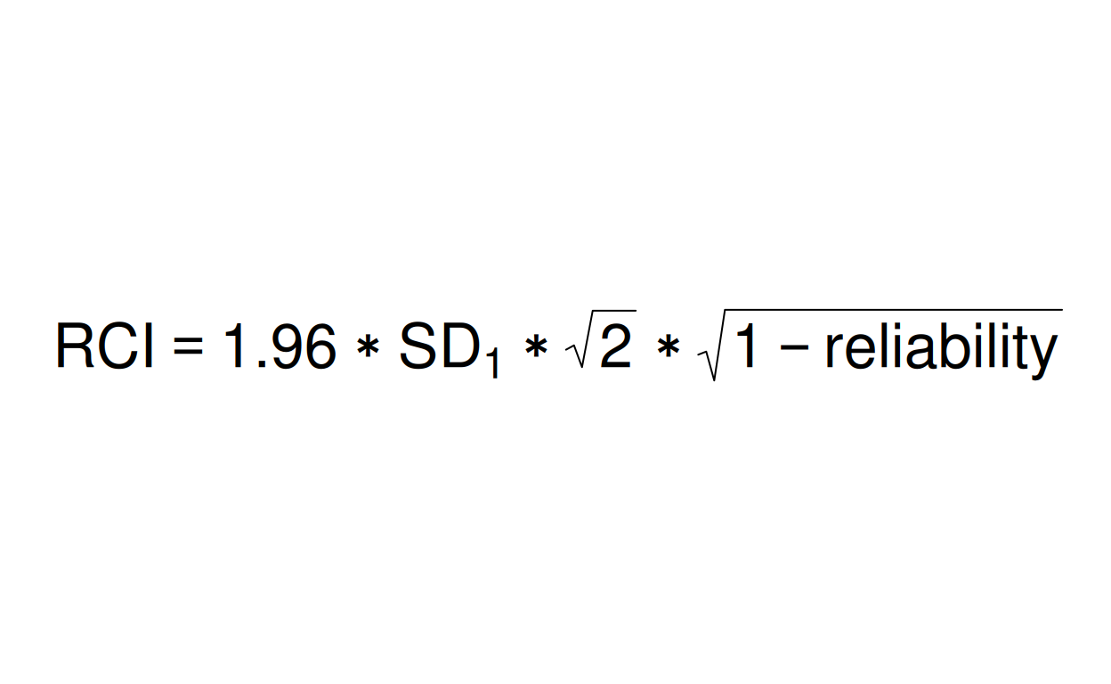
Show code
### this is just the code that creates the "copy to clipboard" function in the code blocks
htmltools::tagList(
  xaringanExtra::use_clipboard(
    button_text = "<i class=\"fa fa-clone fa-2x\" style=\"color: #301e64\"></i>",
    success_text = "<i class=\"fa fa-check fa-2x\" style=\"color: #90BE6D\"></i>",
    error_text = "<i class=\"fa fa-times fa-2x\" style=\"color: #F94144\"></i>"
  ),
  rmarkdown::html_dependency_font_awesome()
)
Introduction
Over many years now I have felt that the way we use the RCI isn’t congruent with its logic. My concern is that it is mostly treated as if it were a referential value which generally means that such values are estimates of a population value. Such values of course should have some exploration of the precision of their estimation through a confidence interval around the estimate and some discussion of likely biases: neither of which seem to happen for the RCI. However, that’s certainly not unique to the RCI!
Many comments on the original paper proposing the RCI and CSC (Jacobson, N. S., Follette, W. C., & Revenstorf, D. (1984). Psychotherapy outcome research: Methods for reporting variability and evaluating clinical significance. Behavior Therapy, 15, 336–352) have focused on the CSC rather than the RCI and on the very real challenges of choosing what are appropriate samples and populations for the “clinical” and “non-clinical” used to get the means and SDs needed to compute a CSC. The original response from Christensen & Mendoza (Christensen, L., & Mendoza, J. L. (1986). A method of assessing change in a single subject: An alteration of the RC index. Behavior Therapy, 17, 305–308.) added the missing square root of two to the equation for the RCI but didn’t comment on whether the two values that determine the RCI, the baseline standard deviation of the scores and the reliability of the measure were to be seen as referential. From my skimpy following of more recent comments seem to be about regression to the mean and other subtleties not what I see as the fundamental issue: that the RCI isn’t an estimate of a population value.
Back in another century I co-authored paper about the RCI & CSC (Evans, C., Margison, F., & Barkham, M. (1998). The contribution of reliable and clinically significant change methods to evidence-based mental health. Evidence Based Mental Health, 1, 70–72. https://doi.org/10.1136/ebmh.1.3.70, Open Access at https://mentalhealth.bmj.com/content/1/3/70) that became quite popular. In it we did comment, I think fairly sensibly, on several issues with the RCSC but we didn’t comment on this issue about the RCI that has grown in importance in my mind since then.
Why do I say that the RCI is not an estimate of a population value? Surely any sample statistic can be regarded as such an estimate? Here’s my logic.
The formula for the RCI starts with the formula for the standard error of a difference between two measurements if there is no change in the true scores and hence any change in the observed scores is only down to unreliability of measurement. That SE is:
\[SE_{diff} = SD_{1}\sqrt{2}\sqrt{1 - reliability}\]
From that, assuming we want the RCI to be such that 95% of such meaningless change would be smaller than the RCI, we have the formula for the RCI:
\[RCI = 1.96 * SD_{1}\sqrt{2}\sqrt{1 - reliability}\]
That 1.96 is the standard Gaussian distribution value such that 95% of a cumulative Gaussian are smaller than it.
My concern is that this means that the RCI isn’t a referential value, it’s an algorithm, a heuristic. The reliability can sensibly be regarded as referential and can be given a confidence interval (CI) around it. However, the SD in that equation is a sample/dataset value, it’s not an estimate of a population value. The RCI tells you that, if the assumptions of Classical Test Theory (CTT) apply, i.e. that you have two observations each per person, that the people are independent of one another (“independence of observations”) and if the true and error variances in the population are Gaussian in distribution then in any situation in which there is no true score change, 95% of the absolute change values, i.e. change up or down as as simple number, not a signed number, will be lower than the RCI. That’s it: the SD is what anchors that assertion in the dataset in question and allows us to see if any change value is “reliable improvement”, “reliable deterioration” or “no reliable change”. It also allows us to see if the proportions of those categories in our dataset differ markedly from the 2.5%, 2.5% and 95% that we would expect if that model applies.
That makes using a referential RCI where SD may be different from that of the dataset you have in front of you incongruent with the logic of the RCI.
That’s the logic and to me it’s irrefutable. What follows explores the impact of this by:
Creating a finite population of data meeting the no change, Gaussian, CTT model
Testing the impact of analysing samples from that population either using a fixed RCI or “per sample” (PS)
Creating censored samples from this population that will have smaller SD than the population, but a non-Gaussian distributions and analysing those using a fixed RCI or “per sample”
Creating samples from this population that are Gaussian in distribution but have varying SDs and analysing these using a fixed RCI or “per sample”
That last is probably the best test of my concern.
Create the population model data
I have opted to simulate a measure with reliability of .8. That means that the population covariance matrix of interest is this.
Show code
### set the reliability you want to simulate
valReliability <- .8
### define the means, (all zero)
vecMeans <- rep(0,3)
### start to design the covariance matrix
covMat <- matrix(rep(0, 3^2),
                 nrow = 3,
                 byrow = TRUE)
### finish the covariance matrix by putting in the variances
diag(covMat) <- c(valReliability,
                  1 - valReliability,
                  1 - valReliability)
### put in column names to make it easy to convert to a tibble
colnames(covMat) <- c("True", "Err1", "Err2")
covMat %>%
  as_tibble() %>%
  flextable() %>%
  colformat_double(digits = 3)
True | Err1 | Err2 |
|---|---|---|
0.800 | 0.000 | 0.000 |
0.000 | 0.200 | 0.000 |
0.000 | 0.000 | 0.200 |
Show code
### set population size for next text and code blocks
populationN <- 20000
The three variables are the true score (which doesn’t change) and the error components. All three are independent of each other hence the off-diagonal covariances are all zero and the variances of the true score of .8 and of the error components of .2 fix the reliability at .8.
This next block of code creates a large (n = 2^{4}) , but finite, population with three variables: True, Err1 and True2. They each have means set to zero, Gaussian distributions and a covariance matrix exactly matching that desired one. (Hence this is a finite population not a sample, if it were a sample the covariances wouldn’t exactly match the desired matrix owing to the randomness of the sampling.)
With those simulated variables I could compute the observed scores and the change values. Here are the first ten observations.
Show code
set.seed(12345) # to get replicable values
### use MASS::mvrnorm() to generate a sample with

MASS::mvrnorm(populationN, vecMeans, covMat, empirical = TRUE) -> tmpMat

### name the columns/variables so we can get them into a tibble
colnames(tmpMat) <- c("True", "Err1", "Err2")
tmpMat %>%
  as_tibble() %>%
  ### now generate the observed scores
  mutate(Obs1 = True + Err1,
         Obs2 = True + Err2,
         Change = Obs2 - Obs1,
         ID = row_number()) -> tibSimDat

tibSimDat %>%
  filter(row_number() < 11) %>%
  flextable() %>%
  colformat_double(digits = 3)
True | Err1 | Err2 | Obs1 | Obs2 | Change | ID |
|---|---|---|---|---|---|---|
0.889 | -0.471 | -0.026 | 0.418 | 0.863 | 0.445 | 1 |
-1.199 | -0.206 | -0.189 | -1.405 | -1.388 | 0.017 | 2 |
-0.393 | 0.061 | -0.185 | -0.332 | -0.578 | -0.246 | 3 |
0.065 | 0.136 | -0.227 | 0.200 | -0.163 | -0.363 | 4 |
-0.532 | -0.201 | 0.022 | -0.734 | -0.511 | 0.223 | 5 |
0.720 | 0.746 | -0.113 | 1.466 | 0.607 | -0.859 | 6 |
-0.785 | -0.046 | 0.359 | -0.832 | -0.426 | 0.405 | 7 |
-1.203 | 0.382 | 0.059 | -0.820 | -1.144 | -0.323 | 8 |
0.512 | 0.026 | -0.062 | 0.538 | 0.449 | -0.089 | 9 |
2.082 | 0.020 | -0.167 | 2.103 | 1.916 | -0.187 | 10 |
Here are the means.
Show code
tibSimDat %>%
  select(-ID) %>%
  summarise(across(everything(), mean)) %>%
  flextable() %>%
  colformat_double(digits = 7)
True | Err1 | Err2 | Obs1 | Obs2 | Change |
|---|---|---|---|---|---|
-0.0000000 | 0.0000000 | -0.0000000 | -0.0000000 | -0.0000000 | -0.0000000 |
OK. All zero to the numeric precision of R on my machine (finite maths means that the values aren’t quite zero, hence the minus signs on some of the means). Now here are the variances.
Show code
tibSimDat %>%
  select(-ID) %>%
  summarise(across(everything(), var)) %>%
  flextable() %>%
  colformat_double(digits = 7)
True | Err1 | Err2 | Obs1 | Obs2 | Change |
|---|---|---|---|---|---|
0.8000000 | 0.2000000 | 0.2000000 | 1.0000000 | 1.0000000 | 0.4000000 |
OK. All as it should be. Here is the correlation matrix across the entire population.
Show code
term | True | Err1 | Err2 | Obs1 | Obs2 | Change | ID |
|---|---|---|---|---|---|---|---|
True | 1.00 | ||||||
Err1 | 0.00 | 1.00 | |||||
Err2 | 0.00 | -0.00 | 1.00 | ||||
Obs1 | 0.89 | 0.45 | -0.00 | 1.00 | |||
Obs2 | 0.89 | -0.00 | 0.45 | 0.80 | 1.00 | ||
Change | 0.00 | -0.71 | 0.71 | -0.32 | 0.32 | 1.00 | |
ID | 0.01 | -0.00 | -0.00 | 0.00 | 0.01 | 0.00 | 1.00 |
Here are the distributions.
Show code
tibSimDat %>%
  pivot_longer(cols = -ID,
               names_to = "Variable") -> tibSimDatLong

tibSimDatLong %>%
  mutate(Variable = ordered(Variable,
                            levels = c("True",
                                       "Err1",
                                       "Err2",
                                       "Obs1",
                                       "Obs2",
                                       "Change"))) -> tibSimDatLong

### get statistics for plots
tibSimDatLong %>%
  group_by(Variable) %>%
  summarise(mean = mean(value),
            median = median(value),
            sd = sd(value)) %>%
  ungroup() -> tmpTibStats

### now plot
ggplot(data = tibSimDatLong,
       aes(x = value)) +
  facet_wrap(facets = vars(Variable),
             ncol = 1,
             scales = "free") +
  geom_histogram(bins = 80) +
  geom_vline(data = tmpTibStats,
             aes(xintercept = mean),
             colour = "green") +
  ggtitle("Histograms of the variables in the population dataset",
          subtitle = "Green reference lines mark the means")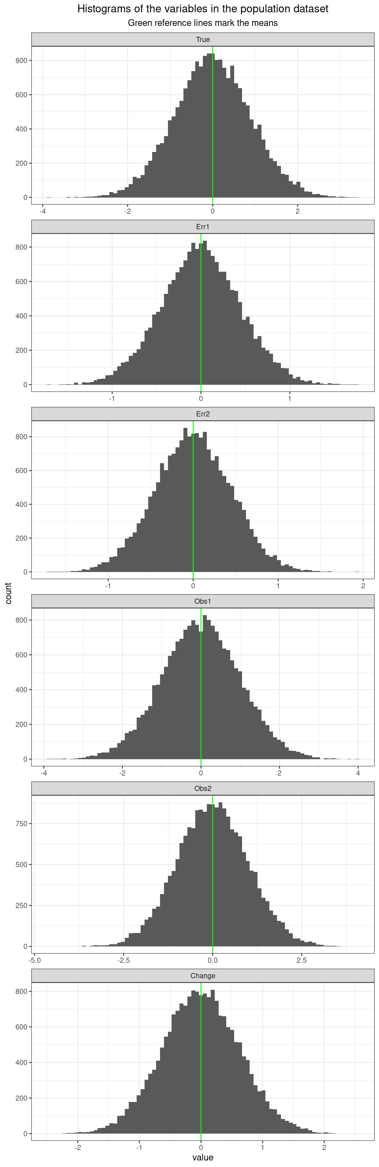
Show code
Drawing samples
OK, the simulation seems OK, let’s use it.
The observed baseline (Obs1) SD is 1 so that gives us an RCI of 1.2396128.
Next I have drawn 20 random samples each of size 2000 from that pseudo population.
Show code
### get the expected counts by multiplying the expected proportions by the sample size
vecExpectedNs <- c(.95, .025, .025) * sampleSize

### now create the samples
tibble(sampleID = 1:nSamples) %>%
  rowwise() %>%
  ### this smples from all the IDs of the rows to determine the values (for those IDs)
  ### that will go into each sample
  ### this has to be done rowwise so you get different selections for each sample
  mutate(IDvals = list(sample(1:populationN, sampleSize, replace = TRUE))) %>%
  ungroup() %>%
  ### OK now unnest those ID values
  unnest_longer(IDvals) %>%
  ### the rest can be done vectorised, i.e. not rowwise()
  mutate(Baseline = pull(tibSimDat[IDvals, "Obs1"]),
         Occ2 = pull(tibSimDat[IDvals, "Obs2"]),
         Change = pull(tibSimDat[IDvals, "Change"])) %>%
  ### get the RCI categorisations
  mutate(absChange = abs(Change),
         RCIcat3way = case_when(
           absChange < valRCI ~ "No reliable change",
           Change >= valRCI ~ "Reliable deterioration",
           Change <= valRCI ~ "Reliable improvement")) -> tibSamples
This is what we see if if we use that RCI based on the baseline SD from whole (finite) population, i.e. from a perfect estimate of the true SD.
Show code
tibSamples %>%
  tabyl(RCIcat3way) %>%
  ### this just deals with an oddity that janitor::tabyl() says its variable is "percent" but
  ### actually gives proportions
  mutate(percent = 100 * percent, # convert to percentages
         percent = sprintf("%4.2f", percent), # get to 2 d.p. and then ... add "%"
         percent = str_c(percent, "%")) %>%
  flextable() %>%
  autofit() %>%
  ### as percent is now a character variable it would align left by default hence ...
  align(j = "percent", align = "right")
RCIcat3way | n | percent |
|---|---|---|
No reliable change | 38,048 | 95.12% |
Reliable deterioration | 1,023 | 2.56% |
Reliable improvement | 929 | 2.32% |
This shows the numbers in each RCI category for each sample but using the population RCI. It also shows the chisquared p value testing the observed numbers against the expected values.
Show code
tibSamples %>%
  group_by(sampleID) %>%
  summarise(nNoRelChange = sum(RCIcat3way == "No reliable change"),
            nRelDet = sum(RCIcat3way == "Reliable deterioration"),
            nRelImp = sum(RCIcat3way == "Reliable improvement")) %>%
  rowwise() %>%
  ### run the chisquared test squashing warnings
  mutate(chisqP = suppressWarnings(chisq.test(as.table(rbind(c(nNoRelChange, nRelDet, nRelImp),
                                                              vecExpectedNs)))$p.value)) %>%
  ungroup() -> tmpTib1

tmpTib1 %>%
  flextable() %>%
  colformat_double(digits = 3) %>%
  ### next two lines do nice conditional background colour formatting
  bg(j = "chisqP", i = ~ chisqP >= .05, bg = "green") %>%
  bg(j = "chisqP", i = ~ chisqP < .05, bg = "red")
sampleID | nNoRelChange | nRelDet | nRelImp | chisqP |
|---|---|---|---|---|
1 | 1,914 | 45 | 41 | 0.548 |
2 | 1,912 | 46 | 42 | 0.638 |
3 | 1,909 | 51 | 40 | 0.565 |
4 | 1,913 | 49 | 38 | 0.429 |
5 | 1,899 | 55 | 46 | 0.817 |
6 | 1,893 | 60 | 47 | 0.602 |
7 | 1,899 | 45 | 56 | 0.740 |
8 | 1,888 | 48 | 64 | 0.407 |
9 | 1,916 | 44 | 40 | 0.458 |
10 | 1,906 | 62 | 32 | 0.073 |
11 | 1,892 | 52 | 56 | 0.820 |
12 | 1,915 | 35 | 50 | 0.258 |
13 | 1,905 | 49 | 46 | 0.912 |
14 | 1,888 | 62 | 50 | 0.516 |
15 | 1,899 | 53 | 48 | 0.938 |
16 | 1,902 | 52 | 46 | 0.902 |
17 | 1,901 | 53 | 46 | 0.881 |
18 | 1,905 | 54 | 41 | 0.591 |
19 | 1,894 | 58 | 48 | 0.725 |
20 | 1,898 | 50 | 52 | 0.980 |
So that shows that all the proportions were as you’d expect given random fluctuations across the samples, and that the chisquared test p value was above .05 for all the samples. The mean p value is 0.64.
What happens if we use the SD of the baseline scores for each sample to compute a per sample RCI? Here are the baseline SDs and the corresponding RCIs per sample just to see how much they vary across the samples.
Show code
sampleID | sampleSD | RCI_PS |
|---|---|---|
1 | 0.9854 | 1.2215 |
2 | 1.0125 | 1.2551 |
3 | 1.0214 | 1.2662 |
4 | 1.0005 | 1.2402 |
5 | 0.9919 | 1.2296 |
6 | 1.0001 | 1.2397 |
7 | 1.0253 | 1.2710 |
8 | 1.0133 | 1.2561 |
9 | 1.0083 | 1.2499 |
10 | 1.0029 | 1.2432 |
11 | 0.9883 | 1.2251 |
12 | 0.9910 | 1.2285 |
13 | 1.0070 | 1.2483 |
14 | 1.0147 | 1.2578 |
15 | 0.9829 | 1.2185 |
16 | 1.0081 | 1.2496 |
17 | 0.9873 | 1.2239 |
18 | 0.9936 | 1.2317 |
19 | 0.9993 | 1.2388 |
20 | 1.0011 | 1.2410 |
And here are the mean baseline SD and RCI values pooling across the 20 samples.
Show code
meanBaselineSD | meanRCI |
|---|---|
1.0017 | 1.2418 |
As you’d expect: pretty close to the population values of 1.0 and 1.2396128
Show code
tibSamples %>%
  ### pull in the per sample RCI so you can do this
  left_join(tibPerSampleStats, by = "sampleID") %>%
  mutate(RCIcat3wayPS = case_when(
    absChange < RCI_PS ~ "No reliable change",
    Change >= RCI_PS ~ "Reliable deterioration",
    Change <= RCI_PS ~ "Reliable improvement")) -> tibSamplesPS

tibSamplesPS %>%
  tabyl(RCIcat3wayPS) %>%
  mutate(percent = 100 * percent,
         percent = sprintf("%4.2f", percent),
         percent = str_c(percent, "%")) %>%
  flextable() %>%
  autofit() %>%
  align(j = "percent", align = "right")
RCIcat3wayPS | n | percent |
|---|---|---|
No reliable change | 38,048 | 95.12% |
Reliable deterioration | 1,027 | 2.57% |
Reliable improvement | 925 | 2.31% |
So pretty much as you’d expect. What are the proportions and chisquared test p values?
Show code
tibSamplesPS %>%
  group_by(sampleID) %>%
  summarise(nNoRelChangePS = sum(RCIcat3wayPS == "No reliable change"),
            nRelDetPS = sum(RCIcat3wayPS == "Reliable deterioration"),
            nRelImpPS = sum(RCIcat3wayPS == "Reliable improvement")) %>%
  rowwise() %>%
  mutate(chisqPPS = suppressWarnings(chisq.test(as.table(rbind(c(nNoRelChangePS, nRelDetPS, nRelImpPS),
                                                              vecExpectedNs)))$p.value)) %>%
  ungroup() -> tmpTibPS

tmpTibPS %>%
  flextable() %>%
  colformat_double(digits = 3) %>%
  bg(j = "chisqPPS", i = ~ chisqPPS >= .05, bg = "green") %>%
  bg(j = "chisqPPS", i = ~ chisqPPS < .05, bg = "red")
sampleID | nNoRelChangePS | nRelDetPS | nRelImpPS | chisqPPS |
|---|---|---|---|---|
1 | 1,902 | 53 | 45 | 0.839 |
2 | 1,918 | 43 | 39 | 0.373 |
3 | 1,920 | 49 | 31 | 0.102 |
4 | 1,913 | 49 | 38 | 0.429 |
5 | 1,891 | 59 | 50 | 0.682 |
6 | 1,894 | 60 | 46 | 0.581 |
7 | 1,913 | 37 | 50 | 0.370 |
8 | 1,894 | 47 | 59 | 0.655 |
9 | 1,919 | 43 | 38 | 0.323 |
10 | 1,907 | 62 | 31 | 0.056 |
11 | 1,884 | 53 | 63 | 0.438 |
12 | 1,911 | 38 | 51 | 0.432 |
13 | 1,906 | 49 | 45 | 0.868 |
14 | 1,894 | 58 | 48 | 0.725 |
15 | 1,890 | 57 | 53 | 0.751 |
16 | 1,904 | 50 | 46 | 0.918 |
17 | 1,894 | 56 | 50 | 0.840 |
18 | 1,902 | 56 | 42 | 0.596 |
19 | 1,894 | 58 | 48 | 0.725 |
20 | 1,898 | 50 | 52 | 0.980 |
So, again as you’d expect, no significant deviations from the expected proportions and the mean p value is: 0.5843, fractionally lower than the 0.64 when using the population RCI across all samples.
Impact truncating baseline scores (creates non-Gaussian distributions)
But what if we censor some of the samples by removing some low and some high baseline scorers and we continue to use the population RCI? This next code block models removing the lowest 25% of baseline scores (perhaps like removing those scoring below the CSC or some other “too low” cut-off in a clinical service) and the highest 10% (referring those clients onward as too high?)
Show code
tibSamples %>%
  summarise(quantiles = list(quantile(Baseline, probs = c(.25, .90)))) %>%
  unnest_wider(quantiles) -> tibQuantiles

tibSamples %>%
  filter(Baseline > tibQuantiles$`25%` & Baseline < tibQuantiles$`90%`) -> tibSamplesCensored

tibSamplesCensored %>%
  group_by(sampleID) %>%
  summarise(SDcensoredPS = sd(Baseline),
            RCIcensoredPS = SDcensoredPS * sqrt(2) * 1.96 * sqrt(1 - valReliability)) %>%
  ungroup() -> tmpTib

tibSamplesCensored %>%
  left_join(tmpTib, by = "sampleID") %>%
  mutate(RCIcat3wayPSCensored = case_when(
  absChange < RCIcensoredPS ~ "No reliable change",
  Change >= RCIcensoredPS ~ "Reliable deterioration",
  Change <= RCIcensoredPS ~ "Reliable improvement")) -> tibSamplesCensored
That gives us overall distribution of baseline scores like this.
Show code
tibSamplesCensored %>%
  summarise(mean = mean(Baseline),
            median = median(Baseline)) -> tmpTibStats

ggplot(data = tibSamplesCensored,
       aes(x = Baseline)) +
  geom_histogram(alpha = .4,
                 bins = 50) +
  geom_vline(xintercept = tmpTibStats$mean,
             colour = "green") +
  geom_vline(xintercept = tmpTibStats$median,
             colour = "blue") +
  geom_vline(xintercept = 0,
             colour = "black",
             linetype = 3) +
  ggtitle("Histogram of baseline scores after truncation",
          subtitle = str_c("Dotted black line is pre-trunctation population mean value",
                           "\nBlue line marks median value after truncation and green marks the mean"))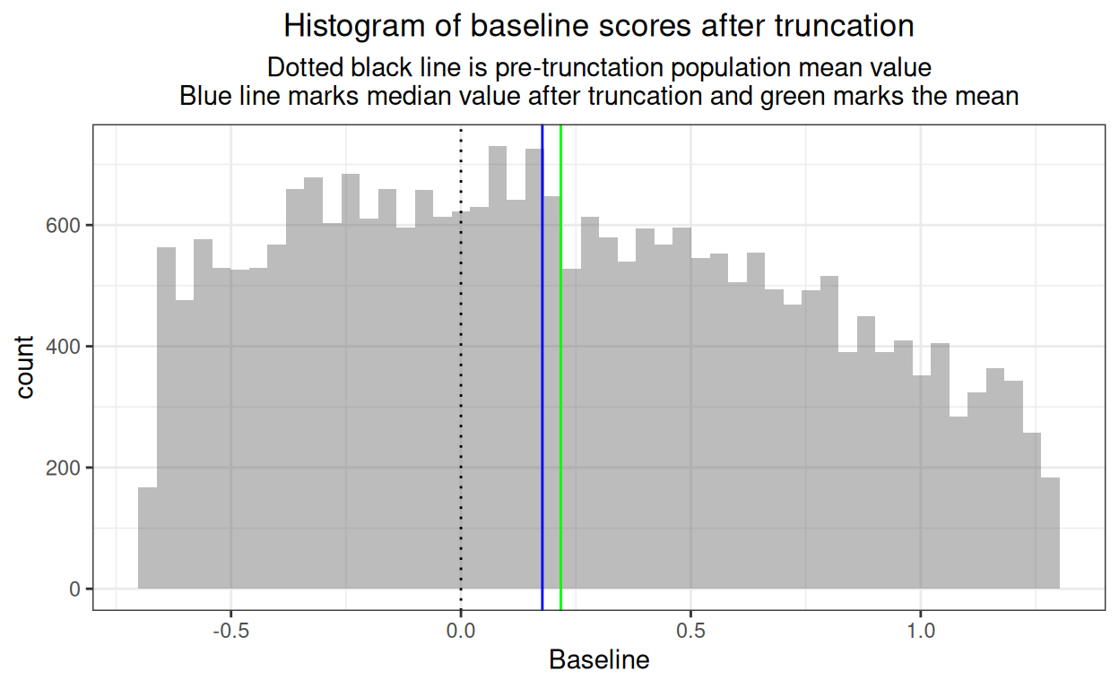
That shows clearly how the mean has shifted and that the distribution is, of course, no longer Gaussian. The individual samples have these statistics (and density plots).
What about the change scores?
Show code
tibSamplesCensored %>%
  summarise(mean = mean(Change),
            median = median(Change)) -> tmpTibStats

ggplot(data = tibSamplesCensored,
       aes(x = Change)) +
  geom_histogram(alpha = .4) +
  geom_vline(xintercept = tmpTibStats$mean,
             colour = "green") +
  geom_vline(xintercept = tmpTibStats$median,
             colour = "blue") +
  geom_vline(xintercept = 0,
             colour = "black",
             linetype = 3) +
  ggtitle("Histogram of change scores after truncation",
          subtitle = str_c("Dotted black line is pre-trunctation population mean value",
                           "\nBlue line marks median value after truncation and green marks the mean"))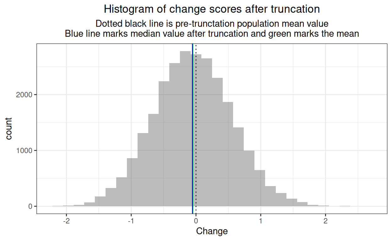
That shows that the change scores still have a distribution close to Gaussian but that its mean has shifted somewhat owing to the asymmetrical truncating.
Show code
tibSamplesCensored %>%
  group_by(sampleID) %>%
  summarise(n = n(),
            meanBaseline = mean(Baseline),
            SDBaseline = sd(Baseline),
            meanChange = mean(Change),
            SDChange = sd(Change),
            RCI_PS = first(RCIcensoredPS),
            Density = list(Baseline)) -> tmpTib

tmpTib %>%
  flextable() %>%
  mk_par(j = "Density",
         value = as_paragraph(
           plot_chunk(value = Density,
                      type = "dens",
                      col = "red")
         )) %>%
  colformat_double(digits = 3)
sampleID | n | meanBaseline | SDBaseline | meanChange | SDChange | RCI_PS | Density |
|---|---|---|---|---|---|---|---|
1 | 1,310 | 0.212 | 0.525 | -0.011 | 0.600 | 0.651 |
|
2 | 1,316 | 0.216 | 0.534 | -0.053 | 0.599 | 0.662 |
|
3 | 1,269 | 0.235 | 0.540 | -0.068 | 0.597 | 0.670 |
|
4 | 1,326 | 0.214 | 0.514 | -0.054 | 0.591 | 0.637 |
|
5 | 1,297 | 0.223 | 0.535 | -0.081 | 0.596 | 0.664 |
|
6 | 1,311 | 0.240 | 0.532 | -0.057 | 0.602 | 0.659 |
|
7 | 1,300 | 0.207 | 0.519 | -0.088 | 0.618 | 0.643 |
|
8 | 1,280 | 0.213 | 0.529 | -0.080 | 0.628 | 0.656 |
|
9 | 1,325 | 0.218 | 0.536 | -0.051 | 0.591 | 0.664 |
|
10 | 1,294 | 0.226 | 0.522 | -0.014 | 0.591 | 0.646 |
|
11 | 1,314 | 0.226 | 0.522 | -0.059 | 0.625 | 0.647 |
|
12 | 1,321 | 0.202 | 0.507 | -0.061 | 0.592 | 0.629 |
|
13 | 1,299 | 0.227 | 0.524 | -0.029 | 0.588 | 0.650 |
|
14 | 1,299 | 0.215 | 0.521 | -0.013 | 0.626 | 0.646 |
|
15 | 1,306 | 0.220 | 0.530 | -0.080 | 0.589 | 0.657 |
|
16 | 1,301 | 0.196 | 0.530 | -0.040 | 0.603 | 0.656 |
|
17 | 1,266 | 0.230 | 0.522 | -0.019 | 0.595 | 0.647 |
|
18 | 1,281 | 0.204 | 0.511 | -0.027 | 0.603 | 0.634 |
|
19 | 1,291 | 0.185 | 0.521 | -0.034 | 0.607 | 0.646 |
|
20 | 1,293 | 0.234 | 0.534 | -0.057 | 0.599 | 0.662 |
|


That shows how the samples have dropped in size from 2000 (though all fairly close to 1300, i.e. 2000 * .65) as you’d expect. That also shows that of course the mean has gone up though again with some variation across the samples as has the SD and so as a linear function of those SD values, do the RCI values now they are computed per sample. Those little density plots, again as you’d expect, don’t show marked differences between samples but, as for the pooled data, are clearly not Gaussian. The impact of the truncation on the change values is less than on baseline values but as it is an asymmetrical truncation it does shift the means a little as seen in the pooled data above. We can see how the RCI computed on the per sample basis, RCI_PS, varies across the samples.
Now using the fixed population RCI on these samples gives us this.
Show code
RCIcat3way | n | percent |
|---|---|---|
No reliable change | 24,931 | 95.89% |
Reliable deterioration | 473 | 1.82% |
Reliable improvement | 595 | 2.29% |
So far fewer than 2.5% show reliable improvement or reliable deterioration as you’d expect given that the truncation has removed the tails of the Gaussian distribution.
Per sample RCI categorisation
However, using the per sample baseline SD values to get RCI values gives this.
Show code
RCIcat3wayPSCensored | n | percent |
|---|---|---|
No reliable change | 18,629 | 71.65% |
Reliable deterioration | 3,258 | 12.53% |
Reliable improvement | 4,112 | 15.82% |
That shows that the proportions achieving reliable change have jumped to way above 2.5% each way as the Gaussian distribution assumptions of the RCI, built into it from its roots in CTT, have markedly overestimated the correct RCI values because the baseline distribution is now far from Gaussian.
OK that underlines that distributions well off from Gaussian will me that RCI won’t give us the proportions we ask it to.
Keeping Gaussian distribution but changing the SD
Show code
vecMultiplier <- c(.7, 1.42)

tibSamples %>%
  mutate(tmpI = as.integer(1 + sampleID %% 2),
         multiplier = vecMultiplier[tmpI],
         newBaseline = Baseline * multiplier,
         newOcc2 = Occ2 * multiplier,
         newChange = newOcc2 - newBaseline,
         newAbsChange = abs(newChange)) %>%
  mutate(RCIcat3wayMultiplied = case_when(
    newAbsChange < valRCI ~ "No reliable change",
    newChange >= valRCI ~ "Reliable deterioration",
    newChange <= valRCI ~ "Reliable improvement")) -> tibSamplesMultiplied
So what happens if we adjust the SD across samples but keep Gaussian distributions? As the baseline scores are centred on zero we can change their SD just by multiplying them by any fixed, non-zero value. Here I have multiplied by one of 0.7 or 1.42 depending on the sample.
Show code
tibSamplesMultiplied %>%
  group_by(sampleID) %>%
  summarise(SDmultiplied = sd(newBaseline),
            RCImultipliedPS = SDmultiplied * 1.96 * sqrt(2) * sqrt(1 - valReliability)) %>%
  ungroup() -> tmpTib

tibSamplesMultiplied %>%
  left_join(tmpTib, by = "sampleID") -> tibSamplesMultiplied

tibSamplesMultiplied %>%
  group_by(sampleID) %>%
  summarise(n = n(),
            multiplier = first(multiplier),
            meanBaseline = mean(newBaseline),
            SDBaseline = first(SDmultiplied),
            meanChange = mean(newChange),
            SDChange = sd(newChange),
            RCI_PS = first(RCImultipliedPS),
            Density = list(Baseline)) -> tmpTib

tmpTib %>%
  select(-c(meanChange, SDChange)) %>%
  flextable() %>%
  mk_par(j = "Density",
         value = as_paragraph(
           plot_chunk(value = Density,
                      type = "dens",
                      col = "red",
                      free_scale = FALSE)
         )) %>%
  colformat_double(digits = 3)
sampleID | n | multiplier | meanBaseline | SDBaseline | RCI_PS | Density |
|---|---|---|---|---|---|---|
1 | 2,000 | 1.420 | 0.007 | 1.399 | 1.735 |
|
2 | 2,000 | 0.700 | 0.000 | 0.709 | 0.879 |
|
3 | 2,000 | 1.420 | -0.008 | 1.450 | 1.798 |
|
4 | 2,000 | 0.700 | 0.016 | 0.700 | 0.868 |
|
5 | 2,000 | 1.420 | 0.008 | 1.408 | 1.746 |
|
6 | 2,000 | 0.700 | 0.014 | 0.700 | 0.868 |
|
7 | 2,000 | 1.420 | -0.006 | 1.456 | 1.805 |
|
8 | 2,000 | 0.700 | -0.006 | 0.709 | 0.879 |
|
9 | 2,000 | 1.420 | 0.032 | 1.432 | 1.775 |
|
10 | 2,000 | 0.700 | -0.004 | 0.702 | 0.870 |
|
11 | 2,000 | 1.420 | -0.015 | 1.403 | 1.740 |
|
12 | 2,000 | 0.700 | 0.005 | 0.694 | 0.860 |
|
13 | 2,000 | 1.420 | 0.034 | 1.430 | 1.773 |
|
14 | 2,000 | 0.700 | -0.014 | 0.710 | 0.880 |
|
15 | 2,000 | 1.420 | -0.006 | 1.396 | 1.730 |
|
16 | 2,000 | 0.700 | 0.020 | 0.706 | 0.875 |
|
17 | 2,000 | 1.420 | -0.039 | 1.402 | 1.738 |
|
18 | 2,000 | 0.700 | -0.014 | 0.696 | 0.862 |
|
19 | 2,000 | 1.420 | -0.055 | 1.419 | 1.759 |
|
20 | 2,000 | 0.700 | 0.001 | 0.701 | 0.869 |
|


That shows the marked change in the SD of the baseline scores, SDBaseline depending on the multiplier and the impact this has on the per sample RCI values (RCI_PS). I think it is almost impossible to see the difference in the SDs in those tiny density plots.
Pooling within the values of the multiplier shows the differences between the distributions of the baseline scores very clearly.
Show code
tibSamplesMultiplied %>%
  select(multiplier, newBaseline) %>%
  pivot_longer(cols = newBaseline) -> tmpTib

tmpTib %>%
  group_by(multiplier) %>%
  summarise(mean = mean(value),
            sd = sd(value)) -> tmpTibMeans

tmpTib %>%
  group_by(multiplier) %>%
  summarise(quantiles = list(quantile(value, probs = c(.05, .25, .75, .95)))) %>%
  unnest_wider(quantiles) %>%
  rename_with(~ str_remove(.x, fixed("%"))) %>%
  rename_with(~ str_c("p", .x)) %>%
  rename(multiplier = pmultiplier) %>%
  pivot_longer(cols = -multiplier,
               names_to = "quantile") -> tmpTibQuantiles

ggplot(data = tmpTib,
       aes(x = value)) +
  facet_wrap(facets = vars(multiplier),
             ncol = 1,
             scale = "fixed") +
  geom_histogram(bins = 50,
                 alpha = .4) +
  geom_vline(data = tmpTibMeans,
             aes(xintercept = mean),
             colour = "blue") +
  geom_vline(data = tmpTibQuantiles,
             aes(xintercept = value),
             colour = "red")+
  ggtitle("Facetted histogram of pooled transformed data facetted by multiplier",
          subtitle = "Blue reference line marks means and red lines mark .05, .25, .75, and .95 quantiles")
Here is the breakdown of the RCI categories using the population RCI of 1.2396128 which we know is now an incorrect RCI as the baseline SDs have been changed.
Show code
tibSamplesMultiplied %>%
  group_by(sampleID) %>%
  summarise(multiplier = first(multiplier),
            SDBaseline = first(SDmultiplied),
            RCI = first(RCImultipliedPS),
            nNoRelChange = sum(RCIcat3wayMultiplied == "No reliable change"),
            nRelDet = sum(RCIcat3wayMultiplied == "Reliable deterioration"),
            nRelImp = sum(RCIcat3wayMultiplied == "Reliable improvement")) %>%
  rowwise() %>%
  mutate(chisqP = suppressWarnings(chisq.test(as.table(rbind(c(nNoRelChange, nRelDet, nRelImp),
                                                              vecExpectedNs)))$p.value)) %>%
  ungroup() -> tmpTib1

tmpTib1 %>%
  flextable() %>%
  colformat_double(digits = 3) %>%
  bg(j = "chisqP", i = ~ chisqP >= .05, bg = "green") %>%
  bg(j = "chisqP", i = ~ chisqP < .05, bg = "red")
sampleID | multiplier | SDBaseline | RCI | nNoRelChange | nRelDet | nRelImp | chisqP |
|---|---|---|---|---|---|---|---|
1 | 1.420 | 1.399 | 1.735 | 1,704 | 149 | 147 | 0.000 |
2 | 0.700 | 0.709 | 0.879 | 1,993 | 3 | 4 | 0.000 |
3 | 1.420 | 1.450 | 1.798 | 1,665 | 176 | 159 | 0.000 |
4 | 0.700 | 0.700 | 0.868 | 1,994 | 2 | 4 | 0.000 |
5 | 1.420 | 1.408 | 1.746 | 1,679 | 153 | 168 | 0.000 |
6 | 0.700 | 0.700 | 0.868 | 1,994 | 4 | 2 | 0.000 |
7 | 1.420 | 1.456 | 1.805 | 1,643 | 162 | 195 | 0.000 |
8 | 0.700 | 0.709 | 0.879 | 1,992 | 3 | 5 | 0.000 |
9 | 1.420 | 1.432 | 1.775 | 1,694 | 155 | 151 | 0.000 |
10 | 0.700 | 0.702 | 0.870 | 1,991 | 4 | 5 | 0.000 |
11 | 1.420 | 1.403 | 1.740 | 1,657 | 177 | 166 | 0.000 |
12 | 0.700 | 0.694 | 0.860 | 1,991 | 5 | 4 | 0.000 |
13 | 1.420 | 1.430 | 1.773 | 1,704 | 157 | 139 | 0.000 |
14 | 0.700 | 0.710 | 0.880 | 1,985 | 9 | 6 | 0.000 |
15 | 1.420 | 1.396 | 1.730 | 1,659 | 156 | 185 | 0.000 |
16 | 0.700 | 0.706 | 0.875 | 1,991 | 3 | 6 | 0.000 |
17 | 1.420 | 1.402 | 1.738 | 1,680 | 166 | 154 | 0.000 |
18 | 0.700 | 0.696 | 0.862 | 1,993 | 6 | 1 | 0.000 |
19 | 1.420 | 1.419 | 1.759 | 1,671 | 176 | 153 | 0.000 |
20 | 0.700 | 0.701 | 0.869 | 1,993 | 2 | 5 | 0.000 |
So all way off from 95% : 2.5% : 2.5%. Here are the mean baseline SD, RCI and p values from the samples pooling within the multiplier.
Show code
multiplier | meanSD | meanRCI | meanP |
|---|---|---|---|
0.70 | 0.70 | 0.87 | 8e-16 |
1.42 | 1.42 | 1.76 | <2e-16 |
Here is the breakdown where the multiplier for the baseline scores was .7.
Show code
RCIcat3wayMultiplied | n | percent |
|---|---|---|
No reliable change | 36,673 | 91.68% |
Reliable deterioration | 1,668 | 4.17% |
Reliable improvement | 1,659 | 4.15% |
Those proportions of reliable change are markedly higher than they should be.
And this shows the same where the multiplier was 1.42.
Show code
RCIcat3wayMultiplied | n | percent |
|---|---|---|
No reliable change | 16,756 | 83.78% |
Reliable deterioration | 1,627 | 8.13% |
Reliable improvement | 1,617 | 8.09% |
Again the proportions are well off from 95% : 2.5% : 2.5%.
Per sample RCI categorisation
Here are the per sample RCIs?
Show code
tibSamplesMultiplied %>%
  mutate(RCIcat3wayMultipliedPS = case_when(
    newAbsChange < RCImultipliedPS ~ "No reliable change",
    newChange >= RCImultipliedPS ~ "Reliable deterioration",
    newChange <= RCImultipliedPS ~ "Reliable improvement")) -> tibSamplesMultiplied

tibSamplesMultiplied %>%
  group_by(sampleID) %>%
  summarise(multiplier = first(multiplier),
            SDBaseline = first(SDmultiplied),
            RCI = first(RCImultipliedPS),
            nNoRelChange = sum(RCIcat3wayMultipliedPS == "No reliable change"),
            nRelDet = sum(RCIcat3wayMultipliedPS == "Reliable deterioration"),
            nRelImp = sum(RCIcat3wayMultipliedPS == "Reliable improvement")) %>%
  rowwise() %>%
  mutate(chisqP = suppressWarnings(chisq.test(as.table(rbind(c(nNoRelChange, nRelDet, nRelImp),
                                                              vecExpectedNs)))$p.value)) %>%
  ungroup() -> tmpTib1

tmpTib1 %>%
  flextable() %>%
  colformat_double(digits = 3) %>%
  bg(j = "chisqP", i = ~ chisqP >= .05, bg = "green") %>%
  bg(j = "chisqP", i = ~ chisqP < .05, bg = "red")
sampleID | multiplier | SDBaseline | RCI | nNoRelChange | nRelDet | nRelImp | chisqP |
|---|---|---|---|---|---|---|---|
1 | 1.420 | 1.399 | 1.735 | 1,902 | 53 | 45 | 0.839 |
2 | 0.700 | 0.709 | 0.879 | 1,918 | 43 | 39 | 0.373 |
3 | 1.420 | 1.450 | 1.798 | 1,920 | 49 | 31 | 0.102 |
4 | 0.700 | 0.700 | 0.868 | 1,913 | 49 | 38 | 0.429 |
5 | 1.420 | 1.408 | 1.746 | 1,891 | 59 | 50 | 0.682 |
6 | 0.700 | 0.700 | 0.868 | 1,894 | 60 | 46 | 0.581 |
7 | 1.420 | 1.456 | 1.805 | 1,913 | 37 | 50 | 0.370 |
8 | 0.700 | 0.709 | 0.879 | 1,894 | 47 | 59 | 0.655 |
9 | 1.420 | 1.432 | 1.775 | 1,919 | 43 | 38 | 0.323 |
10 | 0.700 | 0.702 | 0.870 | 1,907 | 62 | 31 | 0.056 |
11 | 1.420 | 1.403 | 1.740 | 1,884 | 53 | 63 | 0.438 |
12 | 0.700 | 0.694 | 0.860 | 1,911 | 38 | 51 | 0.432 |
13 | 1.420 | 1.430 | 1.773 | 1,906 | 49 | 45 | 0.868 |
14 | 0.700 | 0.710 | 0.880 | 1,894 | 58 | 48 | 0.725 |
15 | 1.420 | 1.396 | 1.730 | 1,890 | 57 | 53 | 0.751 |
16 | 0.700 | 0.706 | 0.875 | 1,904 | 50 | 46 | 0.918 |
17 | 1.420 | 1.402 | 1.738 | 1,894 | 56 | 50 | 0.840 |
18 | 0.700 | 0.696 | 0.862 | 1,902 | 56 | 42 | 0.596 |
19 | 1.420 | 1.419 | 1.759 | 1,894 | 58 | 48 | 0.725 |
20 | 0.700 | 0.701 | 0.869 | 1,898 | 50 | 52 | 0.980 |
Aha, as I thought, all good.
Summary/moral
This confirms that if an RCI is used as a referential criterion when it is based on a sample with SD of the baseline scores that is different from that in your dataset then the proportions in the three RCI categories can be way off from 95% : 2.5% : 2.5 despite your dataset (and the dataset that created the RCI treated as referential) entirely fitting the CTT model behind the RCI.
It also confirms that if you use a per sample RCI in samples from this CTT no-true-change model then the proportions come out much closer to 95% : 2.5% : 2.5%. However, of course they won’t be exactly 95% : 2.5% : 2.5% down to sampling randomness.
It showed that if your dataset has fairly markedly non-Gaussian distributions then the RCI won’t give the proportions you want even in the CTT no-true-change model.
This begs some interesting questions about how much different deviations from Gaussian affect the RCI categorisation and it begs questions about how small a dataset is so small that computing a per sample SD and hence RCI will be no better than using a referential RCI owing to the wide confidence interval around the SD and hence around the RCI to use. Having said that, the logic of the RCI remains one of per sample use so probably for any sensible service dataset (n > 20?) the per sample RCI is probably going to give closer to 95% : 2.5% : 2.5% proportions when baseline SDs vary considerable across different datasets, as they probably do vary across real service datasets.
History
- 27.v.25: finished first publishable version
- 27.v.25: started working on this
web counter
Last updated
28/05/2025 at 13:30