Derangements #2

Follows on from ‘Scores from matching things’

Show code

### this is just the code that creates the "copy to clipboard" function in the code blocks
htmltools::tagList(
  xaringanExtra::use_clipboard(
    button_text = "<i class=\"fa fa-clone fa-2x\" style=\"color: #301e64\"></i>",
    success_text = "<i class=\"fa fa-check fa-2x\" style=\"color: #90BE6D\"></i>",
    error_text = "<i class=\"fa fa-times fa-2x\" style=\"color: #F94144\"></i>"
  ),
  rmarkdown::html_dependency_font_awesome()
)

Show code

as_tibble(list(x = 1,
               y = 1)) -> tibDat

ggplot(data = tibDat,
       aes(x = x, y = y)) +
  geom_text(label = "Derangements #2",
            size = 20,
            colour = "red",
            angle = 30,
            lineheight = 1) +
  xlab("") +
  ylab("") +
  theme_bw() +
  theme(panel.grid.major = element_blank(),
        panel.grid.minor = element_blank(),
        panel.border = element_blank(),
        panel.background = element_blank(),
        axis.line = element_blank(),
        axis.text = element_blank(),
        axis.ticks = element_blank()) 

Updated to add contact me 11.ix.22

In my last post here, Scores from matching things I gave the background to the probabilities of achieving certain scores on matching tasks by chance alone to help explain the perhaps counter-intuitive finding that matching four or more things correctly is unlikely by chance alone at p < .05 regardless of the number of objects to be matched.

This just adds a bit more to that, mostly as plots and complements both that Rblog post and an “ordinary” blog post, Sometimes n=4 is enough.

What I wanted was to show how rapidly the probabilities of achieving any particular score stabilise to an asymptotic value as n increases. Here we are for n from 4 to 15 and scores from 4 to 10.

Show code

### create some functions (as in previous post)
all.derangements <- function(n){
  cumprob <- prob <- number <- term <- score <- rev(0:n)
  for (m in 1:n) {
    i <- m+1
    s <- n-m
    term[i] <- ((-1)^(m))/(factorial(m))
  }  
  term[1] <- 1
  for (i in 0:n) {
    s <- i+1
    prob[s] <- (sum(term[1:s]))/factorial(n-i)
  }
  number <- factorial(n)*prob
  for (s in 0:n) {
    m <- n-s
    i <- m+1
    cumprob[i] <- sum(prob[1:i])
  }
  tmp <- cbind(n, score,number,prob,cumprob)
  tmp
}

p.derange.score <- function(score,n){
  if (score > n) stop("Score cannot be greater than n")
  if (score == (n-1)) stop ("Score cannot be n-1")
  cumprob <- prob <- term <- rev(0:n)
  for (m in 1:n) {
    i <- m+1
    s <- n-m
    term[i] <- ((-1)^(m))/(factorial(m))
  }  
  term[1] <- 1
  for (i in 0:n) {
    s <- i+1
    prob[s] <- (sum(term[1:s]))/factorial(n-i)
  }
  for (s in 0:n) {
    m <- n-s
    i <- m+1    
    cumprob[i] <- sum(prob[1:i])
  }
  cumprob[n+1-score]
}

### now let's go a bit further
### get all the possible scores for n from 4 to 30
lapply(4:30, FUN = all.derangements) -> tmpList
### I always forget this nice little bit of base R and I'm a bit surprised that there doesn't seem to be a nice tidyverse alternative
do.call(rbind.data.frame, tmpList) %>%
  as_tibble() -> tmpTib
### this was just to produce some tables for my blog post at https://www.psyctc.org/psyctc/2022/07/23/sometimes-n4-is-enough/
# tmpTib %>% 
#   write_csv(file = "derangements.csv")

### ditto
# 1:14 %>% 
#   as_tibble() %>%
#   rename(n = value) %>%
#   mutate(PossibleWays = factorial(n),
#          PossibleWays = prettyNum(PossibleWays, big.mark = ",")) %>%
#   write_csv(file = "numbers.csv")

### but Vectorizing the function seemed cleaner so ...
Vectorize(FUN = all.derangements) -> All.derangements
All.derangements(4:14) -> tmpList
### back to the do.call() just for the tables 
# do.call(rbind, tmpList) %>%
#   as_tibble() %>%
#   filter(score == 4) %>%
#   select(n, number) %>%
#   mutate(number = prettyNum(number, big.mark = ",")) %>%
#   write_csv("correct.csv")

# do.call(rbind, tmpList) %>%
#   as_tibble() %>%
#   filter(score == 4) %>%
#   mutate(totalPerms = factorial(n)) %>%
#   select(-prob) %>%
#   select(n, totalPerms, everything()) %>%
#   write_csv("final.csv")
  

### OK, now for this Rblog post!
All.derangements(4:15) -> tmpList
do.call(rbind, tmpList) %>%
  as_tibble() %>%
  filter(score > 3 & score < 11) %>%
  mutate(score = ordered(score,
                         levels = 4:10)) -> tmpTib

ggplot(data = tmpTib,
       aes(x = n, y = cumprob, colour = score, group = score)) +
  geom_point() +
  geom_line() +
  scale_x_continuous(breaks = 3:15,
                     minor_breaks = 3:15,
                     limits = c(3, 15)) +
  ylab("p") +
  theme_bw()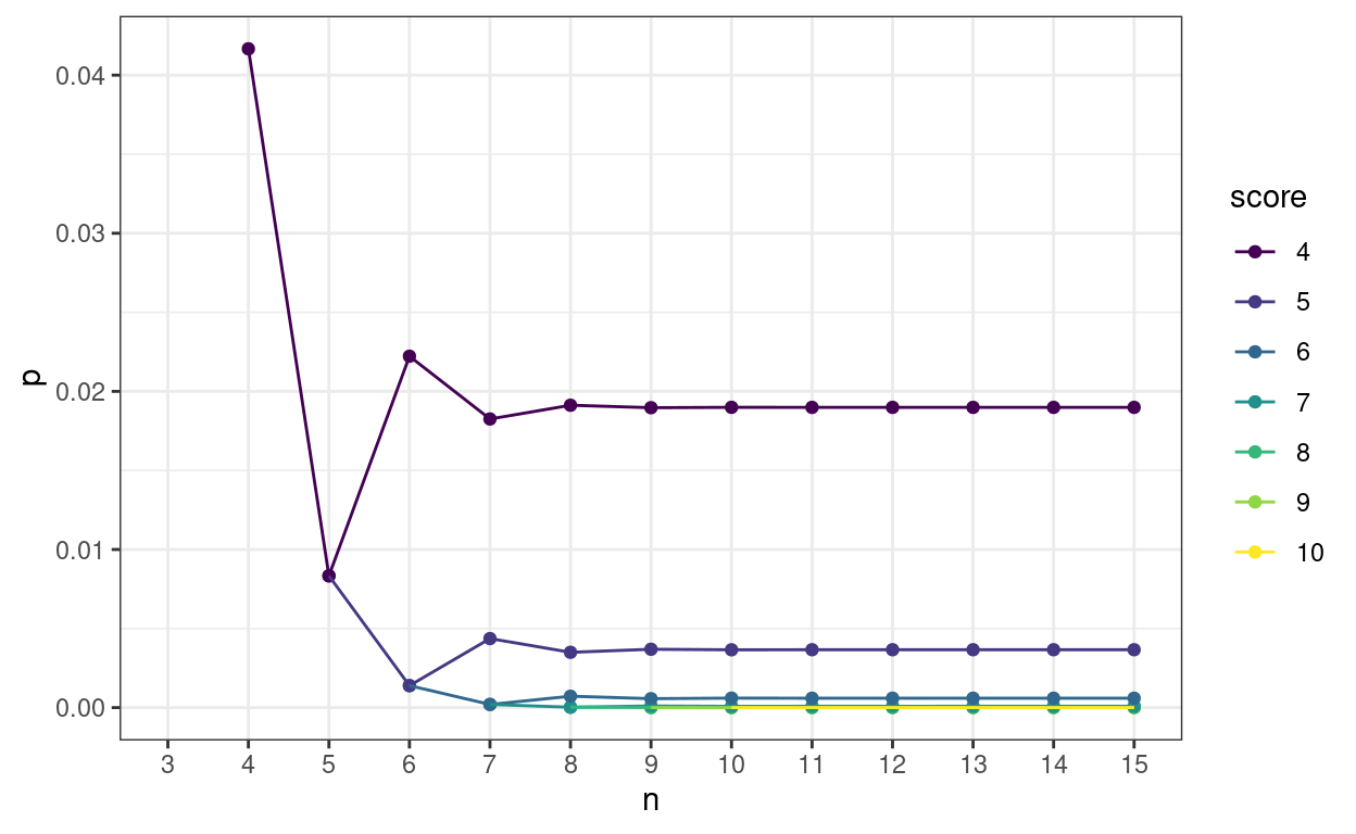 

Here’s the same on a log10 y axis to separate the p values for the higher scores.

Show code

ggplot(data = tmpTib,
       aes(x = n, y = cumprob, colour = score, group = score)) +
  geom_point() +
  geom_line() +
  scale_x_continuous(breaks = 3:15,
                     minor_breaks = 3:15,
                     limits = c(3, 15)) +
  scale_y_continuous(trans = "log10") +
  ylab("p") +
  theme_bw()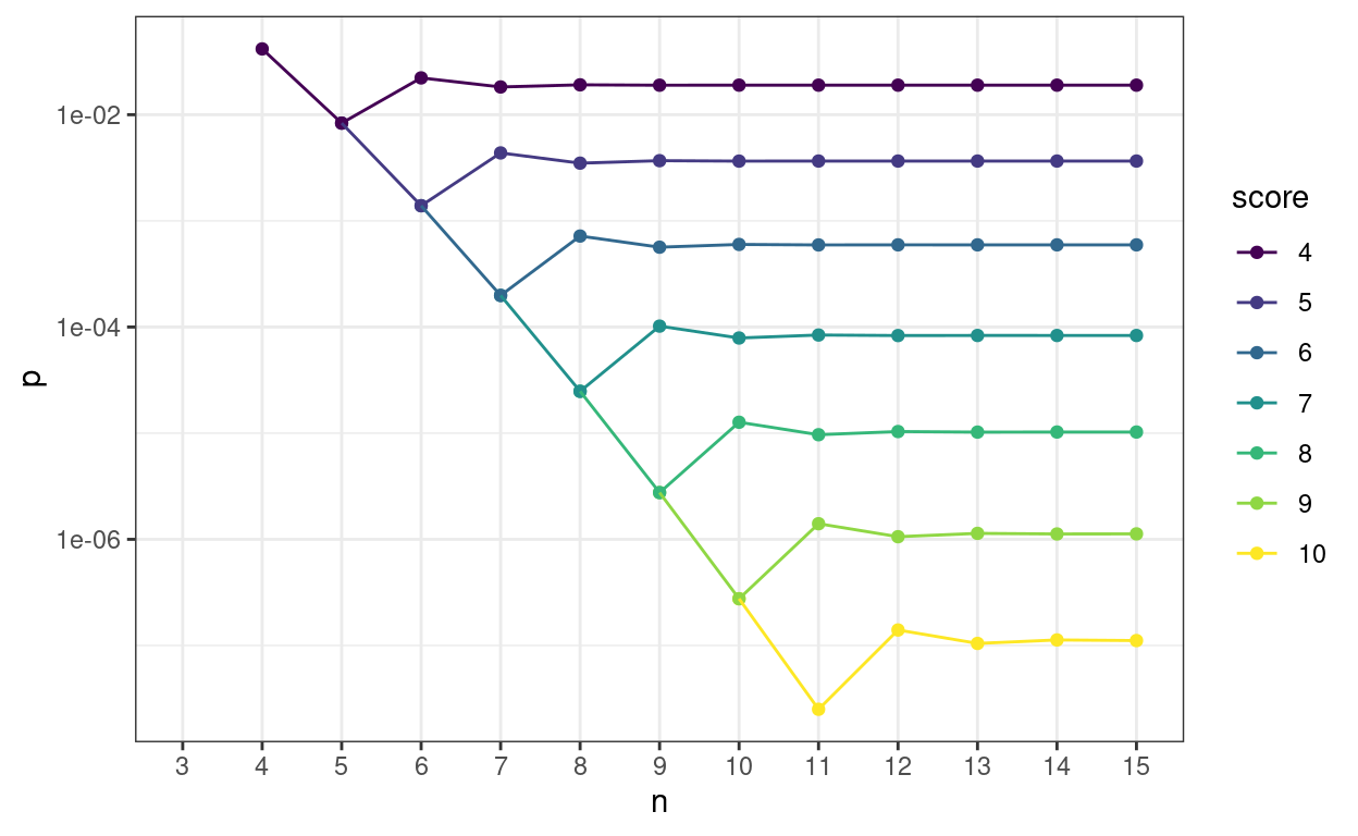 

This next table shows how rapidly p values of real interest stabilise. The table is ordered by number of objects (n) within score. The column p is the probability of getting that score or better by chance alone, diffProb is the absolute change in that p value from the one for the previous n, diffPerc is the difference as a percentage of the previous p value. diffProbLT001 flags when the change in absolute p vaue is below .001 at which point I think in my realm any further precision is spurious. However, diffLT1pct flags when the change in p value is below 1% of the previous p value just in case someone wants that sort precise convergence.

Show code

All.derangements(4:20) -> tmpList
do.call(rbind, tmpList) %>%
  as_tibble() %>%
  filter(score > 3 & score < 11)  -> tmpTib


### just working out how stable the p values get how soon
tmpTib %>%
  arrange(score) %>%
  group_by(score) %>%
  mutate(diffProb = abs(cumprob - lag(cumprob)),
         diffProbLT001 = if_else(diffProb < .001, "Y", "N"),
         diffPerc = 100 * diffProb /lag(cumprob),
         diffLT1pct = if_else(diffPerc < 1, "Y", "N")) %>% 
  ungroup() %>%
  select(-c(number, prob)) %>%
  rename(p = cumprob) %>%
  select(score, everything()) %>%
  as_hux() %>%
  set_position("left") %>% # left align the whole table
  set_bold(row = everywhere, col = everywhere) %>% # everything into bold
  set_align(everywhere, everywhere, "center") %>% # everything centred
  set_align(everywhere, 1:2, "right") %>% # but now right justify the first two columns
  map_text_color(by_values("Y" = "green")) %>% # colour matches by text recognition
  map_text_color(by_values("N" = "red"))

score	n	p	diffProb	diffProbLT001	diffPerc	diffLT1pct
4	4	0.0417
4	5	0.00833	0.0333	N	80	N
4	6	0.0222	0.0139	N	167	N
4	7	0.0183	0.00397	N	17.9	N
4	8	0.0191	0.000868	Y	4.76	N
4	9	0.019	0.000154	Y	0.807	Y
4	10	0.019	2.31e-05	Y	0.122	Y
4	11	0.019	3.01e-06	Y	0.0158	Y
4	12	0.019	3.44e-07	Y	0.00181	Y
4	13	0.019	3.53e-08	Y	0.000186	Y
4	14	0.019	3.28e-09	Y	1.73e-05	Y
4	15	0.019	2.78e-10	Y	1.47e-06	Y
4	16	0.019	2.17e-11	Y	1.15e-07	Y
4	17	0.019	1.57e-12	Y	8.29e-09	Y
4	18	0.019	1.06e-13	Y	5.59e-10	Y
4	19	0.019	6.71e-15	Y	3.53e-11	Y
4	20	0.019	3.99e-16	Y	2.1e-12	Y
5	5	0.00833
5	6	0.00139	0.00694	N	83.3	N
5	7	0.00437	0.00298	N	214	N
5	8	0.0035	0.000868	Y	19.9	N
5	9	0.00369	0.000193	Y	5.52	N
5	10	0.00366	3.47e-05	Y	0.941	Y
5	11	0.00366	5.26e-06	Y	0.144	Y
5	12	0.00366	6.89e-07	Y	0.0188	Y
5	13	0.00366	7.95e-08	Y	0.00217	Y
5	14	0.00366	8.2e-09	Y	0.000224	Y
5	15	0.00366	7.65e-10	Y	2.09e-05	Y
5	16	0.00366	6.52e-11	Y	1.78e-06	Y
5	17	0.00366	5.12e-12	Y	1.4e-07	Y
5	18	0.00366	3.72e-13	Y	1.02e-08	Y
5	19	0.00366	2.52e-14	Y	6.87e-10	Y
5	20	0.00366	1.59e-15	Y	4.35e-11	Y
6	6	0.00139
6	7	0.000198	0.00119	N	85.7	N
6	8	0.000719	0.000521	Y	262	N
6	9	0.000565	0.000154	Y	21.5	N
6	10	0.0006	3.47e-05	Y	6.15	N
6	11	0.000593	6.31e-06	Y	1.05	N
6	12	0.000594	9.65e-07	Y	0.163	Y
6	13	0.000594	1.27e-07	Y	0.0214	Y
6	14	0.000594	1.48e-08	Y	0.00248	Y
6	15	0.000594	1.53e-09	Y	0.000258	Y
6	16	0.000594	1.44e-10	Y	2.42e-05	Y
6	17	0.000594	1.23e-11	Y	2.07e-06	Y
6	18	0.000594	9.67e-13	Y	1.63e-07	Y
6	19	0.000594	7.04e-14	Y	1.19e-08	Y
6	20	0.000594	4.78e-15	Y	8.04e-10	Y
7	7	0.000198
7	8	2.48e-05	0.000174	Y	87.5	N
7	9	0.000102	7.72e-05	Y	311	N
7	10	7.88e-05	2.31e-05	Y	22.7	N
7	11	8.41e-05	5.26e-06	Y	6.68	N
7	12	8.31e-05	9.65e-07	Y	1.15	N
7	13	8.33e-05	1.48e-07	Y	0.179	Y
7	14	8.32e-05	1.97e-08	Y	0.0236	Y
7	15	8.32e-05	2.3e-09	Y	0.00276	Y
7	16	8.32e-05	2.39e-10	Y	0.000287	Y
7	17	8.32e-05	2.25e-11	Y	2.7e-05	Y
7	18	8.32e-05	1.93e-12	Y	2.32e-06	Y
7	19	8.32e-05	1.53e-13	Y	1.83e-07	Y
7	20	8.32e-05	1.12e-14	Y	1.34e-08	Y
8	8	2.48e-05
8	9	2.76e-06	2.2e-05	Y	88.9	N
8	10	1.27e-05	9.92e-06	Y	360	N
8	11	9.67e-06	3.01e-06	Y	23.7	N
8	12	1.04e-05	6.89e-07	Y	7.12	N
8	13	1.02e-05	1.27e-07	Y	1.23	N
8	14	1.03e-05	1.97e-08	Y	0.192	Y
8	15	1.02e-05	2.62e-09	Y	0.0256	Y
8	16	1.02e-05	3.08e-10	Y	0.003	Y
8	17	1.02e-05	3.22e-11	Y	0.000314	Y
8	18	1.02e-05	3.04e-12	Y	2.96e-05	Y
8	19	1.02e-05	2.62e-13	Y	2.55e-06	Y
8	20	1.02e-05	2.07e-14	Y	2.02e-07	Y
9	9	2.76e-06
9	10	2.76e-07	2.48e-06	Y	90	N
9	11	1.4e-06	1.13e-06	Y	409	N
9	12	1.06e-06	3.44e-07	Y	24.6	N
9	13	1.14e-06	7.95e-08	Y	7.51	N
9	14	1.12e-06	1.48e-08	Y	1.3	N
9	15	1.13e-06	2.3e-09	Y	0.204	Y
9	16	1.13e-06	3.08e-10	Y	0.0273	Y
9	17	1.13e-06	3.62e-11	Y	0.00322	Y
9	18	1.13e-06	3.8e-12	Y	0.000337	Y
9	19	1.13e-06	3.6e-13	Y	3.2e-05	Y
9	20	1.13e-06	3.11e-14	Y	2.76e-06	Y
10	10	2.76e-07
10	11	2.51e-08	2.51e-07	Y	90.9	N
10	12	1.4e-07	1.15e-07	Y	458	N
10	13	1.05e-07	3.53e-08	Y	25.3	N
10	14	1.13e-07	8.2e-09	Y	7.85	N
10	15	1.11e-07	1.53e-09	Y	1.36	N
10	16	1.11e-07	2.39e-10	Y	0.215	Y
10	17	1.11e-07	3.22e-11	Y	0.0289	Y
10	18	1.11e-07	3.8e-12	Y	0.00341	Y
10	19	1.11e-07	4e-13	Y	0.000359	Y
10	20	1.11e-07	3.8e-14	Y	3.41e-05	Y

Do contact me if this interests you and if you might want to use the method with real data.

Visit count

free web page counter