[This post cross-links to entries in the glossary for our OMbook (Evans, C., & Carlyle, J. (2021). Outcome measures and evaluation in counselling and psychotherapy (1st ed.). SAGE Publishing.), particularly the one on the Bonferroni correction!]
The correction
The Bonferroni correction is a very simple and easy to understand “correction” for the multiple tests problem. That problem is that when we do more than one null hypothesis test the risk of at least one false positive result climbs above the nominal criterion (usually .05 or 1 in 20). See the glossary entry here.
The Bonferroni correction is to reset the alpha criterion, that conventional .05, to a smaller number that exactly cancels out the increased risk of any false positives across your tests. If k is the number of tests and \(\alpha\) is your criterion the Bonferroni correction is actually to use a criterion of \(\alpha/k\) so if you are using the conventional \(\alpha\) of .05 and you were doing two tests you would only consider either test statistically significant if the observed p value were \(\leqslant .025\).
So staying with an \(\alpha\) of .05 we get this table of Bonferroni corrected \(\alpha\) levels (correctedAlpha) to use for different numbers of tests.
Show code
k | alphaDesired | correctedAlpha |
|---|---|---|
1 | 0.0500 | 0.0500 |
2 | 0.0500 | 0.0250 |
3 | 0.0500 | 0.0167 |
4 | 0.0500 | 0.0125 |
5 | 0.0500 | 0.0100 |
6 | 0.0500 | 0.0083 |
7 | 0.0500 | 0.0071 |
8 | 0.0500 | 0.0063 |
9 | 0.0500 | 0.0056 |
10 | 0.0500 | 0.0050 |
Why does this work?
Under the general null hypothesis of no population effect for any of the k tests the probability of any one test giving a false positive is always your chosen \(\alpha\) i.e. .05 usually. The probability of all of tests not giving a false positive must be \(.95^{k}\) and the risk of at least one false positive must be one minus that risk, i.e. \(1 - .95^{k}\), hence the multiple tests problem
Show code
k | alphaDesired | riskFalsePositives |
|---|---|---|
1 | 0.05 | 0.05 |
2 | 0.05 | 0.10 |
3 | 0.05 | 0.14 |
4 | 0.05 | 0.19 |
5 | 0.05 | 0.23 |
6 | 0.05 | 0.26 |
7 | 0.05 | 0.30 |
8 | 0.05 | 0.34 |
9 | 0.05 | 0.37 |
10 | 0.05 | 0.40 |
That’s the problem: the risk of at least one false positive is going up rapidly with the number of tests despite the general null hypothesis, i.e. that nothing is going on for any of the tests, being true of the population.
The Bonferroni correction works because it is replacing the \(\alpha\) for a single test with \(\alpha/k\) so the risk of at least one false positive is \(1-(\alpha/k)^{k}\). This next table shows that using the Bonferroni correction, i.e. testing against \(\alpha/k\) keeps the overall risk of at least one false positive (\(1-(\alpha/k)^{k}\)) at .05.
Show code
k | alphaDesired | correctedAlpha | BonfRiskFalsePositives |
|---|---|---|---|
1 | 0.05 | 0.05 | 0.05 |
2 | 0.05 | 0.03 | 0.05 |
3 | 0.05 | 0.02 | 0.05 |
4 | 0.05 | 0.01 | 0.05 |
5 | 0.05 | 0.01 | 0.05 |
6 | 0.05 | 0.01 | 0.05 |
7 | 0.05 | 0.01 | 0.05 |
8 | 0.05 | 0.01 | 0.05 |
9 | 0.05 | 0.01 | 0.05 |
10 | 0.05 | 0.01 | 0.05 |
What’s the catch?
The correction is fine to keep the overall (experimentwise or studywise) false positive risk at \(\alpha\) given the general null hypothesis being true for the population from which it is assumed the sample data came. The problem is that the correction is inevitably costing a lot of statistical power so unless you can easily increase the size of your samples your risk of failing to detect as statistically significant one or more effects that may be non-null in the population.
This plot shows power for a simple two group t-test with a population effect size of .5 against sample size and how using the Bonferroni correction with different numbers of tests drops the power below that for a single test (using \(\alpha = .05\)).
Show code
getPower <- function(n, d, alpha){
  pwr::pwr.t.test(n = n, d = d, sig.level = alpha)$power
}
# getPower(100, .5, .05)

tibble(n = 10:100,
       k = list(1:10)) %>%
  unnest_longer(k) %>%
  mutate(power = getPower(n, d = .5, alpha = .05 / k),
         k = factor(k,
                    levels = 1:10)) -> tibPower

ggplot(data = tibPower,
       aes(x = n, y = power, colour = k, group = k)) +
  geom_point() +
  geom_line() +
  # geom_hline(yintercept = .05,
  #            linetype = 3) +
  # geom_hline(yintercept = getPower(100, .5, .05),
  #            colour = "red") +
  # ggtitle("Power for two-group t-test and effect size .5 against n",
  #         paste0("Separate lines for different numbers of tests (k) with Bonferroni correction",
  #                "\nDotted reference line at .05 and red line at power for single test and n = 100"))
    ggtitle("Power for two-group t-test and effect size .5 against n",
          "Separate lines for different numbers of tests (k) with Bonferroni correction")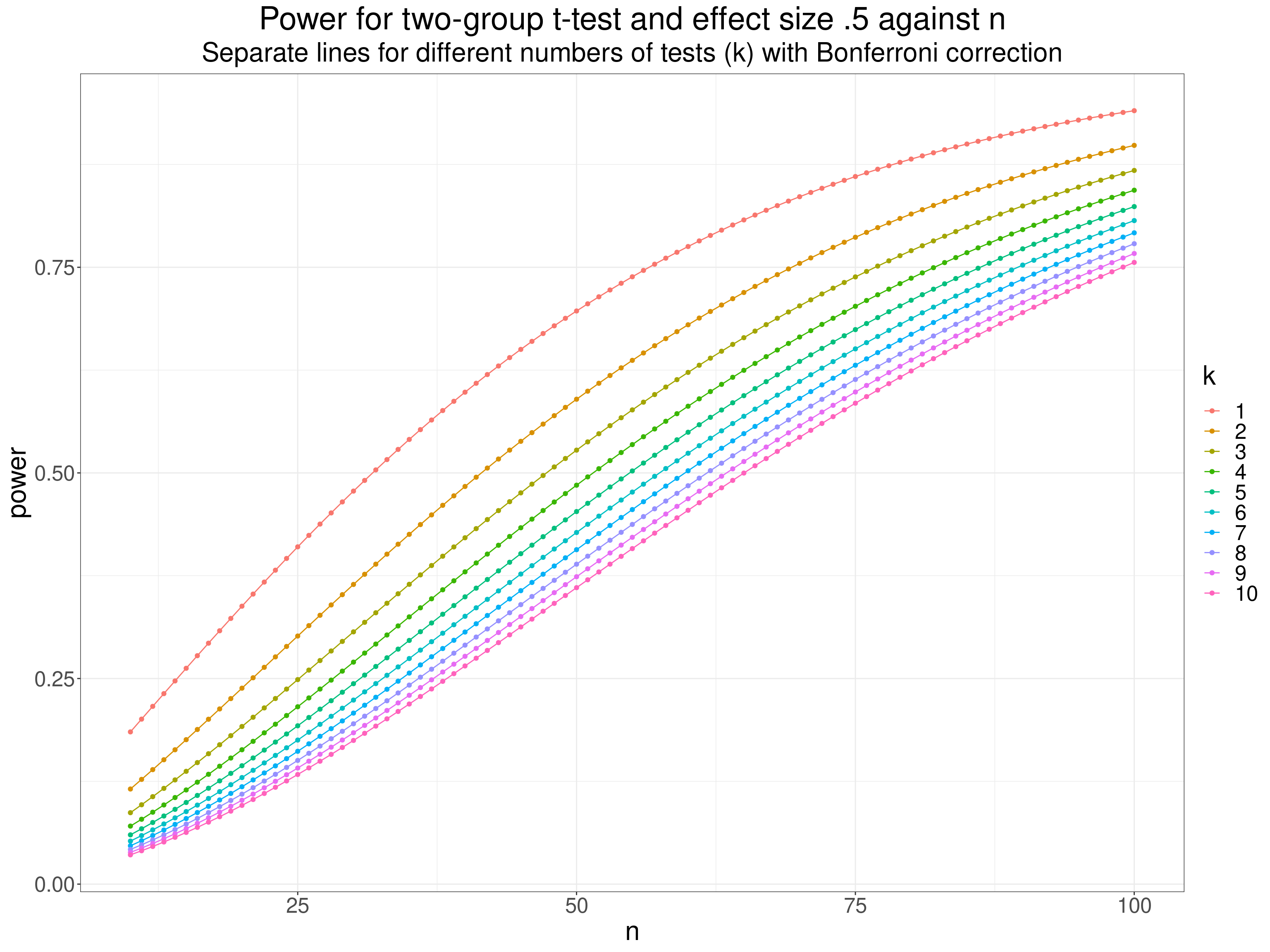
Another way to show this for the same model is show the effect of increasing numbers of tests for a few selected sample sizes (in facets).
Show code
tibPower %>%
  filter(n %in% c(10, 25, 50, 100)) %>%
  mutate(doubleK = as.double(k)) -> tibPower2

ggplot(data = tibPower2,
       aes(x = doubleK, y = power)) +
  facet_wrap(facets = vars(n),
             nrow = 2) +
  geom_line(linewidth = 1) +
  geom_point(aes(colour = k),
             size = 3) +
  scale_x_continuous("k",
                     breaks = 1:10) +
  ggtitle("Power against number of tests",
          subtitle = "Facets for samples sizes")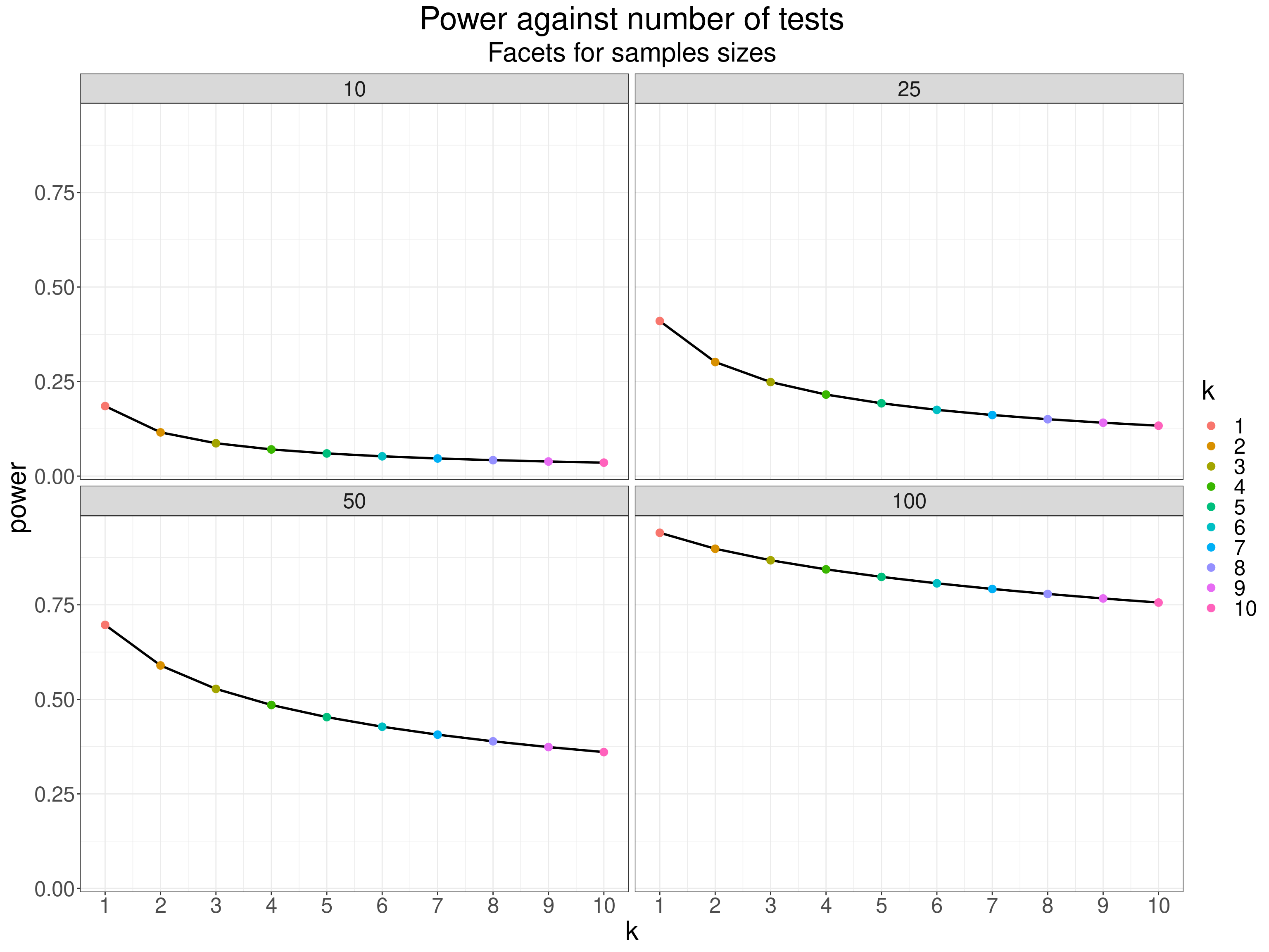
So the catch is that if the general null model is incorrect and you do have non-null effects in the population then you are losing real statistical power to detect these effects using the Bonferroni correction as the number of tests you apply goes up. There are alternatives to the Bonferroni correction that can balance this inevitable trade off of power for retention of the experimentwise false positive rate involving different population models but the basic trade off is inescapable. This leads into real issues about when we might take what approach to the multiple tests problem including accepting that the overall, experimentwise, reportwise, false positive rate may be well above your conventional \(\alpha\) but that you will accept that because you are more worried about failing to detect individual effects as significant than about the rising overall false positive risk. Given that most papers report more than one test the issue is probably too often either ignored completely, or dealt with simply by using the Bonferroni correction without much or any discussion of the cost to statistical power. Sadly, I confess that I’ve done both of those wriggles. One problem is that discussing the issues properly in the discussion section of a paper is not easy to do clearly for all levels of statistical knowledge in the readers and, perhaps more sadly, probably pulls away some of the pretence that we have clear and easy answers to these trade offs. I have created a shiny app, using the t-test example, to show the trade off between correction of the false positive rate against loss of statistical power, see here.
Though it’s easy to show the multiple tests problem for NHSTs (Null Hypothesis Significance Tests) the issues apply equally when using confidence intervals(CIs)/estimation rather than the NHST paradigm though perhaps the sense of definite implications in the move from the maths to the English language is a bit less savage when using CIs/estimation.