Chris (Evans) R SAFAQ: Holm-Bonferroni method

Chris Evans

I wrote this to help me create an entry in my glossary (that I started for our OMbook). This complements my post here in the Rblog about the Bonferroni correction and my Shiny app here that shows the costs of the simple Bonferroni correction in terms of statistical power

Like the Bonferroni method, from which it was developed by Holm, the Holm-Bonferroni nethod is a way of mitigating the multiple tests issue/problem. The objective, as with the simple Bonferroni method, is to try to keep at a fixed level, usually .05, the risk of any statistically significant findings arising within a set of tests even when there are no effects in the population. This is known to researchers and statisticians as maintaining the False Discovery Rate (FDR) across those tests, the family-wise FDR.

Holm-Bonferroni nethod extends the simple Bonferroni method to reduce the loss of statistical power that the Bonferroni method brings.

This post is really here just to show how the method works.

In what follows I start by simulating sampling from a general population null model with 30 Gaussian variables each with population variance 1.0 and means zero and making the variables independent of one another (i.e. all inter-variable correlations at the population level zero). That is just a starting point though it illustrates the multiple tests issue.

Then to demonstrate how the H-B method works I tweaked that population model to include some variables with non-null means. This brings statistical power into the simulation and, with appropriate sample size and non-zero population means for these variables the simulation could demonstrate the H-B method gaining statistical power over the simple Bonferroni method.

In this simulation the test was a single sample t-test testing then null model that the population mean for the variable was zero but the principles are exactly the same for any null hypothesis test being conducted across multiple hypotheses. In fact, the tests don’t even have to be the same tests, you could apply the logic to all the null hypothesis tests of any sort across a paper. Having said that I’ve never seen that done and the whole issue of handling the multiple tests problem only ever seems to come up for “families” of the same tests within a paper, e.g. of a set of sociodemographic predictors against early termination or whether different clinicians in a service have different early termination rates … etc.

Global population null model

Show code

set.seed(123456)
n <- 1500

vecMeans <- c(rep(0, nVars))
matCov <- matrix(rep(0, nVars * nVars),
                 nrow = nVars)
diag(matCov) <- rep(1, nVars)

matDat <- MASS::mvrnorm(n = n, mu = vecMeans, Sigma = matCov)
colnames(matDat) <- str_c("V", 
                          sprintf("%02.0f", 1:nVars))
as_tibble(matDat,
          .name_repair) -> tibDatNull

tibDatNull %>%
  pivot_longer(cols = everything(),
               names_to = "PredVar") %>%
  group_by(PredVar) %>%
  summarise(mean = mean(value),
            p = t.test(value)$p.value) %>%
  arrange(p) -> tibPvalsNull

alphaBonferroni = .05 / nVars

I generated my data using the mvrnorm() function in the MASS package which makes it trivially easy to simulate taking samples from Gaussian population distributions with any defined set of population means and covariances. I set the covariance matrix to independence so all the variables are uncorrelated with each other at the population level.

In this simulation I set n = 1500 and simulated 30 variables each with population variance 1 and population mean (the null) of zero.

So the Bonferroni test value is .05/30 = 0.0016667 and this is modelling the global null so the population means for all 30 variables are zero. As noted above, my test on the simulated sample was a single sample t-test on each variable. As noted above, the principles apply to absolutely any null hypothesis significance test (NHST), this use of the t-test is just nice and easy to write and very CPU efficient, not that you have to worry about that on modern machines!

Here is a plot of our p values for this sample.

Show code

ggplot(data = tibPvalsNull,
       aes(x = reorder(PredVar,
                       p),
           y = p)) +
  geom_point() +
  geom_line(group = 1) +
  geom_hline(yintercept = .05,
             linetype = 3) +
  geom_hline(yintercept = alphaBonferroni,
             linetype = 3,
             colour = "red") +
  scale_y_continuous("P values",
                     breaks = seq(0, 1, .1)) +
  xlab("Predictor variables") +
  theme(axis.text.x = element_text(angle = 70, 
                                   hjust = 1))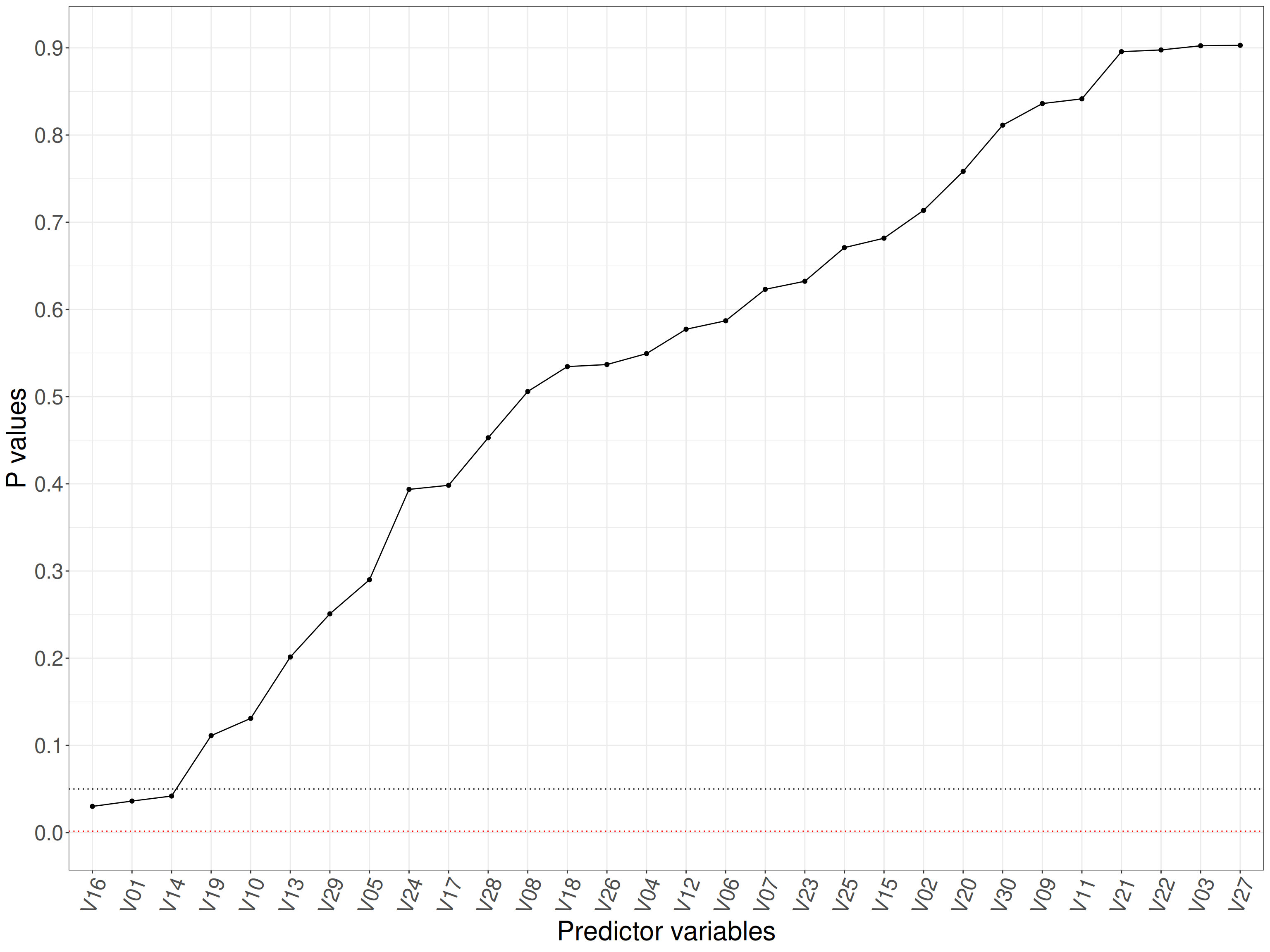

The multiple tests issue makes it likely with that many variables that we might see “false positives”: p values smaller than our conventional criterion of .05 that have arisen by chance. The smallest five p values from this simulation are these.

Show code

tibPvalsNull %>%
  filter(row_number() <= 5) %>%
  flextable() %>%
  bg(i = ~ p < .05,
     j = 3,
     bg = "green")

PredVar	mean	p
V16	-0.05899866	0.03008122
V01	-0.05360094	0.03619070
V14	-0.05147037	0.04191134
V19	0.04019983	0.11121251
V10	0.03873931	0.13102130

So we have 3 statistically significant predictor if we ignore the multiple tests challenge.

However, if we use the Bonferroni criterion of significance, 0.0016667 we have, as we want given that we know this dataset was created as a sample from a population in which the global null is true, of no variables with means statistically significantly different from zero.

Simulate non-null case

The point of the Holm-Bonferroni method is that it mitigates the very conservative nature of the simple Bonferroni “correction” so it increases the statistical power of testing so we want some non-null, i.e. non zero, population means to illustrate this.

Show code

set.seed(12345)
vecNonZeroMeans <- rev(c(.02, .03, .06, .075, .08, .09, .1, .13, .2, .25))
vecMeans <- c(vecNonZeroMeans,
              rep(0, nVars - length(vecNonZeroMeans)))
matCov <- matrix(rep(0, nVars * nVars),
                 nrow = nVars)
diag(matCov) <- rep(1, nVars)

matDat <- MASS::mvrnorm(n = n, 
                        mu = vecMeans, 
                        Sigma = matCov)

colnames(matDat) <- str_c("V", 
                          sprintf("%02.0f", 1:nVars))
as_tibble(matDat) -> tibDatNonNull

tibDatNonNull %>%
  pivot_longer(cols = everything(),
               names_to = "PredVar") %>%
  group_by(PredVar) %>%
  summarise(mean = mean(value),
            p = t.test(value)$p.value) %>% 
  mutate(popMean = vecMeans) %>%
  select(PredVar, popMean, everything())  %>%
  arrange(p) -> tibPvalsNonNull

What I have done now is to simulate taking a sample from a population where the variable means are not all zero but include population means of 0.25, 0.2, 0.13, 0.1, 0.09, 0.08, 0.075, 0.06, 0.03, 0.02 for the first five variables (but zero for the remaining 20 variables). As the simulation has set the population variances to 1 these variables have effect size differences from zero of the same values as those means.

Here is a plot of our p values for a sample from that population.

Show code

ggplot(data = tibPvalsNonNull,
       aes(x = reorder(PredVar,
                       p),
           y = p)) +
  geom_point() +
  geom_line(group = 1) +
  geom_hline(yintercept = .05,
             linetype = 3) +
  geom_hline(yintercept = alphaBonferroni,
             linetype = 3,
             colour = "red") +
  scale_y_continuous("P values",
                     breaks = seq(0, 1, .1)) +
  xlab("Predictor variables") +
  theme(axis.text.x = element_text(angle = 70, 
                                   hjust = 1))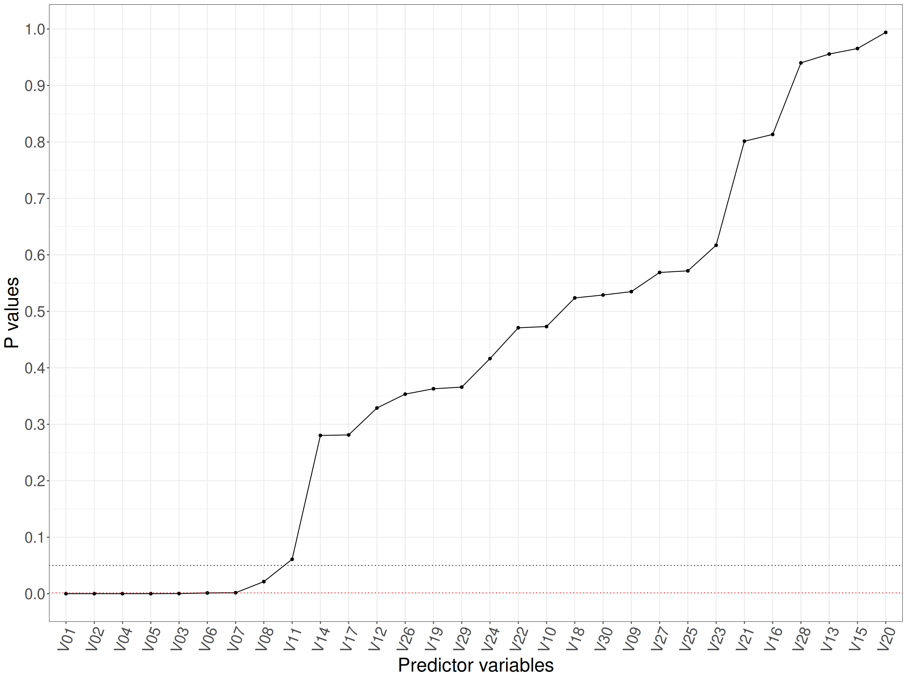

The smallest ten p values are these.

Show code

tibPvalsNonNull %>%
  filter(row_number() <= 10) %>%
  flextable()

PredVar	popMean	mean	p
V01	0.250	0.30663675	0.000000000000000000000000000004489338
V02	0.200	0.20587503	0.000000000000008081070545747541243535
V04	0.100	0.14057877	0.000000064376120557721848234281221673
V05	0.090	0.13464959	0.000000088240152958377926422006080464
V03	0.130	0.09614595	0.000204095438438757552325128474812743
V06	0.080	0.08373301	0.001272635995415240511147159097049553
V07	0.075	0.08475325	0.001672923748795048307091981598659913
V08	0.060	0.05804323	0.021364405716811852437020391448641021
V11	0.000	0.04793579	0.060920853348219672351859799164230935
V14	0.000	0.02835146	0.280217454837319468463618932219105773

Show code

tibPvalsNonNull %>%
  filter(p < .05) %>%
  mutate(alphaBonferroni = alphaBonferroni,
         BonfSignificant = if_else(p < alphaBonferroni,
                                   "Sig",
                                   "NS")) -> tibPlt05

So if we again ignore the multiple tests challenge we have 8 statistically significant at the conventional .05 alpha criterion. (It’s called alpha as part of the whole NHST paradigm.)

Show code

tibPlt05 %>%
  flextable() %>%
  bg(i = ~ BonfSignificant == "Sig",
     bg = "green")

PredVar	popMean	mean	p	alphaBonferroni	BonfSignificant
V01	0.250	0.30663675	0.000000000000000000000000000004489338	0.001666667	Sig
V02	0.200	0.20587503	0.000000000000008081070545747541243535	0.001666667	Sig
V04	0.100	0.14057877	0.000000064376120557721848234281221673	0.001666667	Sig
V05	0.090	0.13464959	0.000000088240152958377926422006080464	0.001666667	Sig
V03	0.130	0.09614595	0.000204095438438757552325128474812743	0.001666667	Sig
V06	0.080	0.08373301	0.001272635995415240511147159097049553	0.001666667	Sig
V07	0.075	0.08475325	0.001672923748795048307091981598659913	0.001666667	NS
V08	0.060	0.05804323	0.021364405716811852437020391448641021	0.001666667	NS

However, if we use the Bonferroni criterion of significance, 0.0016667 we have 6 variables with means statistically significantly different from zero (though 10). This failure to detect five variables as having non zero means might be sampling luck, or that the sample size was simply too small to give the necessary power to detect the smaller population means but it is definitely hampered by the Bonferroni correction being very conservative with that new alpha value of 0.0016667. The point of the Holm-Bonferroni method is not to lose as much statistical power as you do using the Bonferroni correction itself and it does that by applying different alpha levels to different variables in a sensible way.

Holm-Bonferroni method

It is a step-by-step procedure. First the p values are put in increasing order. Then the first, i.e. the smallest p value, is tested against the Bonferroni criterion, then the second is tested using the Bonferroni approach but eliminating the first variable so the new p value criterion is .05 / (nVars - 1), then the next is tested against the criterion of .5 / (nVars - 2). You are basically applying the Bonferroni correction to the diminishing number of predictor variables. As soon as you hit a non-significant p value you stop the process and any remaining tests are declared not statistically significant.

Here’s how that worked for my simulated data.

Show code

tibPvalsNonNull %>%
  mutate(alphaBonferroni = alphaBonferroni,
         alphaHolmB = if_else(row_number() == 1,
                              alphaBonferroni,
                              .05 / (nVars - row_number() - 1)),
         ### messy correction to the two last ones: 0/0 and -.05
         alphaHolmB = if_else(is.infinite(alphaHolmB) | alphaHolmB < 0,
                              .05, # arbitrary, you're never going to use it!
                              alphaHolmB),
         BonfSignificant = if_else(p < alphaBonferroni,
                                   "Sig",
                                   "NS"),
         HolmBonfSig = if_else(p < alphaHolmB,
                               "Sig",
                               "NS"),
         ### now get the sequential stopping rule into this
         HolmBonfSig = if_else(row_number() > 1 &
                                 lag(HolmBonfSig)== "NS",
                               "Stopped",
                               HolmBonfSig),
         ### now blank out the alphaHolmB values where the process had stopped
         alphaHolmB = if_else(HolmBonfSig == "Stopped",
                              NA_real_,
                              alphaHolmB)) %>%
  flextable() %>%
  bg(i = ~ BonfSignificant == "Sig",
     j = 7,
     bg = "green") %>%
  bg(i = ~ HolmBonfSig == "Sig",
     j = 8,
     bg = "green")

PredVar	popMean	mean	p	alphaBonferroni	alphaHolmB	BonfSignificant	HolmBonfSig
V01	0.250	0.3066367528	0.000000000000000000000000000004489338	0.001666667	0.001666667	Sig	Sig
V02	0.200	0.2058750274	0.000000000000008081070545747541243535	0.001666667	0.001851852	Sig	Sig
V04	0.100	0.1405787748	0.000000064376120557721848234281221673	0.001666667	0.001923077	Sig	Sig
V05	0.090	0.1346495903	0.000000088240152958377926422006080464	0.001666667	0.002000000	Sig	Sig
V03	0.130	0.0961459459	0.000204095438438757552325128474812743	0.001666667	0.002083333	Sig	Sig
V06	0.080	0.0837330054	0.001272635995415240511147159097049553	0.001666667	0.002173913	Sig	Sig
V07	0.075	0.0847532486	0.001672923748795048307091981598659913	0.001666667	0.002272727	NS	Sig
V08	0.060	0.0580432344	0.021364405716811852437020391448641021	0.001666667	0.002380952	NS	NS
V11	0.000	0.0479357856	0.060920853348219672351859799164230935	0.001666667		NS	Stopped
V14	0.000	0.0283514628	0.280217454837319468463618932219105773	0.001666667		NS	Stopped
V17	0.000	0.0272549052	0.281138937242195185994830808340338990	0.001666667		NS	Stopped
V12	0.000	-0.0252007213	0.328811953585823490975315053219674155	0.001666667		NS	Stopped
V26	0.000	-0.0243192336	0.353390731738433161446266694838413969	0.001666667		NS	Stopped
V19	0.000	-0.0237593475	0.362881134637285884814161818212596700	0.001666667		NS	Stopped
V29	0.000	-0.0227688667	0.365830648622573972872373815334867686	0.001666667		NS	Stopped
V24	0.000	0.0208459098	0.416352767944992985249541561643127352	0.001666667		NS	Stopped
V22	0.000	0.0187954683	0.470882125745471280531262436852557585	0.001666667		NS	Stopped
V10	0.020	-0.0176639717	0.473077131835015429750512794271344319	0.001666667		NS	Stopped
V18	0.000	-0.0161434715	0.523788338512839346527982797852018848	0.001666667		NS	Stopped
V30	0.000	0.0162922358	0.528924650518951322553107274870853871	0.001666667		NS	Stopped
V09	0.030	0.0157193497	0.534932605646283088063341892848256975	0.001666667		NS	Stopped
V27	0.000	-0.0150174602	0.568842845952657327757151506375521421	0.001666667		NS	Stopped
V25	0.000	0.0148515160	0.571732583539841243691626004874706268	0.001666667		NS	Stopped
V23	0.000	-0.0123673349	0.617053958310734618208925894577987492	0.001666667		NS	Stopped
V21	0.000	0.0065312969	0.801284356558894517164048920676577836	0.001666667		NS	Stopped
V16	0.000	0.0062075082	0.813304624866326486554157781938556582	0.001666667		NS	Stopped
V28	0.000	-0.0018837081	0.940039262242496231891664137947373092	0.001666667		NS	Stopped
V13	0.000	-0.0014187013	0.955681797459660864468844465591246262	0.001666667		NS	Stopped
V15	0.000	-0.0011164479	0.965408395976037336794206566992215812	0.001666667		NS	Stopped
V20	0.000	-0.0001889352	0.994034047698343026233658292767358944	0.001666667		NS	Stopped

That shows that for this particular sample, sample size and set of non-null population means the Holm-Bonferroni method was sufficiently less conservative than the simple Bonferroni method as it classified one more of the non-null variables as statistically significantly different from zero and I hope, more to the point here, that it illustrates how the method works, relaxing the alpha criterion a little for each variable after variable with the lowest p value (if that was low enough to be significant using the Bonferroni criterion), continuing that until it hits a non-significant finding when the process stops and all remaining variables are classified as non-significant.

Summary

Well, there you have it: the fairly simple process behind the method that somewhat mitigates the loss of statistical power inherent in the simple Bonferronic method while, like it, preserving the family-wise false discovery rate.
I am not statistician enough to be able to explain why it will always work and always be no more conservative than the simple Bonferroni method but I trust that there are proofs of that.
There are methods that gain even more improvement in statistical power, the Holm-Šidák method and the Hochberg and Hommel procedures, but I think that they can fail in the presence of non-zero relationships (correlations) between the variables, at least that seems to be true for the Hochberg procedure according to https://en.wikipedia.org/wiki/Holm%E2%80%93Bonferroni_method#Adjusted_p-values but now I am getting out of my depth and beyond what I think is needed for all but the most determined worshippers of the NHST in our field as I think we are getting to that point where the seductive clarity of the maths might be blinding us to thinking carefully about what our null hypotheses and alternatives really are and whether the NHST is what we need!

Visit count

free counter

Dates

20.ix.26 Remembered to add this Dates section!
18.ix.26 First Created

Last updated

Show code

cat(paste(format(Sys.time(), "%d/%m/%Y"), "at", format(Sys.time(), "%H:%M")))

18/09/2026 at 19:20

Holm-Bonferroni method

Global population null model

Simulate non-null case

Holm-Bonferroni method

Summary

Dates

Last updated

Reuse

Citation