Principal Component Analysis (PCA)

A “dimension reduction” method of rearranging multivariate data. It’s been used for decades in psychology to look at the correlations between items of a questionnaire (where it’s often, wrongly for pedants like me, referred to as a factor analysis!) It’s also something you may come across in genetic studies now as its ability to simplify data from many people on very, very many gene loci is valuable. I think it may also be used in MRI (Magnetic Resonance Imaging) again for the ability to simplify data from umpteen “voxels” in a scan.

Details #

The basic maths is that if you have scores on a lot of variables, typically the k items of a questionnaire (k is usually used for that number), then if you have values for all k items for more than k + 1 observations (typically independent, i.e. not repeated, completions of a questionnaire) then the maths of PCA will rearrange the data to give you “component scores” on k “principal components”. So you seem to have translated one n by k matrix of numbers: how does that help?

The crucial thing is that new matrix has the nice properties that the first principal component (PC) accounts for the most possible variance across all the items and n values. (Hence “principal” I assume.) The second component accounts for the most variance after that first component is removed … and so on until the last (kth) component. The other crucial thing is that the maths also ensures (depends upon) all k components being “orthogonal” to one another: uncorrelated.

I find the analogy of taking a map of k cities of some country and taking measurements of how far each one is from some random point on the map, then taking another random point and measuring the distance to each city from that point; keep going until you have at least k + sets of measurements of those distances from each of the random points. That n by k matrix of numbers isn’t very informative. However, if you push the numbers into a PCA (any statistics package will do this for you and in a split second on modern computers) you will find that you have two PCs with numbers and the remaining k – 2 components will all be zeros (if you have measured the distances near perfectly).

That’s because you started with a 2D reality and the magic of PCA has recovered it for you. The PCs won’t necessarily be aligned North to South and East to West but the first will be orthogonal to the second (at right angles to it) and the first will actually lie along the line of maximum variance in the values for each city.

It’s not a perfect analogy to what goes on conducting PCAs on questionnaire data but it is a way of understanding what PCA is doing: it’s mapping data, good enough for our purposes. I think it may be pretty close to what is going on in constructing an MRI scan (but that would be using distances in 3D not 2D).

Clearly the variance across the items in a questionnaire is not neatly 2D or 3D. Here PCA is more like using a set of distances by road between cities. Now we have a reality (those distances) based n a 2D reality (the locations of the cities, curvature of the Earth is ignorable here!). However, now that reality is a bit hidden by the torturousness of the different roads between the cities. Here, PCA will probably recover a map that is not grossly out from the 2D map but it will be distorted from that and it might be that it would show a non-trivial third dimension in the PCA created by the torturousness.

That’s not a mad analogue of what goes on when PCA is used to understand responses on questionnaires: we are looking to see if there is an underlying structure in the participants’ responses reflecting what we think may be a commonality across people. However, we know that any such commonality will be embedded within other systematic and random issues affecting how individuals respond.

Sometimes it may be clear that some simple dimensions are being recovered. For example, for the Hospital Anxiety and Depression Scales (HADS) with seven anxiety oriented items and seven depression oriented items a PCA tends to show most of the variance in the first two components. (Yes, I know I use this for my examples again and again but that’s because it’s nice and simple!)

Here is a “scree plot” for HADS responses showing the proportion of the total variance across the 14 items (and from 433 participants).

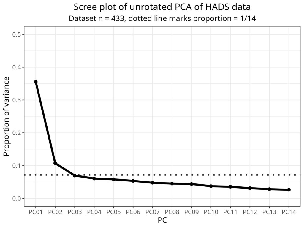
That suggests that, indeed, much of the variance in that 14×433 matrix of participants’ responses is in the first two components.

Then we go a bit beyond the basics of PCA and “rotate” the PCA (imagine rotating a map perhaps to get magnetic north upwards, or to have the way you are moving upwards). You can also use a bit more maths let go of the orthogonality for those first two components (as we may suspect that “anxiety” and “depression” are not generally uncorrelated phenomena). That gets us this loading matrix:

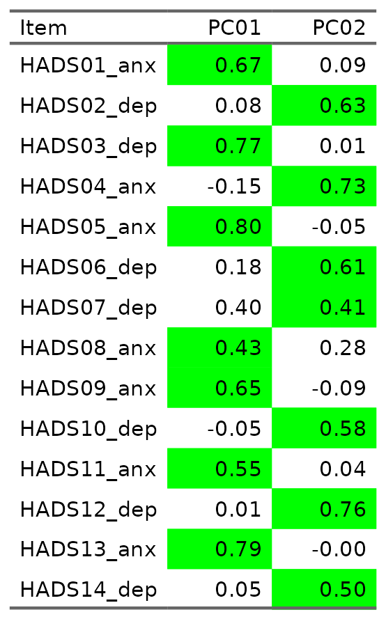
I have followed the usual convention in this sort of psychometric analysis and marked loadings stronger than .4 in green. We can see that the items map, i.e. load more than .4, to the two principal components as we would expect from the design of the HADS: all the anxiety items map to one component, all the depression items map to the other. The output also told me that the correlation between those two rotated components was .45.

Summary #

PCA is a way of reorganising multidimensional data, i.e. in our field, typically a dataset of numeric responses to items on multi-item questions from a good number of participants. It is often referred to as a “factor analysis” and the output has much in common with that of factor analyses. However, it is simply reorganising the data to simplify it, it implies no presumed structure of common and unique factors and has, in principle, no distributional assumptions. It has, probably largely for reasons of methodolatry rather than strong logic, largely fallen out of favour in psychometric analysis of questionnaire data in our field while at the same time it has become much more important in analysing CT and MRI scan data and genomic data where its strength of simplifying even very high dimensional data have become very important.