Oversimplifying only a little, IRT, with Classical Test Theory (CTT), makes the two main, and often warring, approaches to analysing the data from responses to multi-item questionnaires.
Details #
CTT assumes that the numbers allocated to responses, i.e. 0 for “Not at all”, 1 for “Only occasionally”, 2 for “Sometimes” and so on, can be treated as interval scaling numbers i.e. can be treated as if the difference between 0 and 1 is the same as between 1 and 2 even if it can’t be assumed that the zero is a true zero or that 2 is twice the magnitude of 1. That is to assume that the numbers are like Centigrade or Fahrenheit temperature measurement which have those properties (unlike measuring temperature in Kelvin where zero is a true zero and unlike measurement of height or weight or blood concentrations all of which have the true zero and ration scaling). It builds on that with a some other key assumptions.
IRT by contrast makes no such assumptions about mapping responses to numbers but gives a way to map the responses to levels on the presumed latent variable. There are many different IRT methods but all work by assuming that items can be selected that form a unidimensional scale (i.e. only relate to one latent variable on which people differ though contaminated with “error”) and then assuming that each item has an “item response” profile (hence the “IR” in “IR”). The basic assumption in IRT is that people differ on the latent variable the scale seeks to measure: some have more of the variable, some less and that the items differ in how it becomes more likely that people with more of the latent variable are more likely to agree to the item. (Or less if the item is cued the other way.)
That’s the model for binary response, i.e. “yes”/”no” items, the mappings, these item response profiles are more complex where there are more than one response category for each item but the theory is similar.
Again simplifying but only minimally, within IRT there are host of different methods for binary and for short ordinal responses. Most of them assume that the response curve has a parametric form, i.e. that it can be defined by one, two or even three “parameters”: values that define the shapes of the curves. The exception is Mokken scaling which only assumes that the curves are monotonic (see Mokken scaling).
Simplifying yet again, yet again only minimally there are three main models:
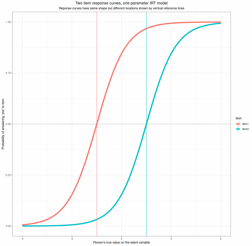
- One parameter per item response (per response level for short ordinal responses). This parameter defines where the item (item response) is on the latent variable and is usually defined by the score on the latent (unmeasurable) variable at which people with that score have a 50:50 probability of answering “yes” or “no”. Here are two items differing only in their location parameter.
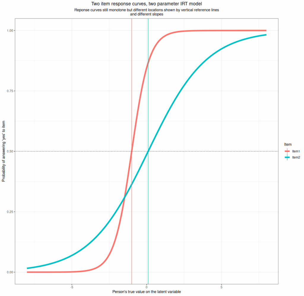
- Two parameter per item models. These have the same location parameter but a second parameter which controls the strength of the relationship between the probability of positive responding against the respondent’s position on the latent varaible, i.e. the slope of the item response curve. Here’s an example.
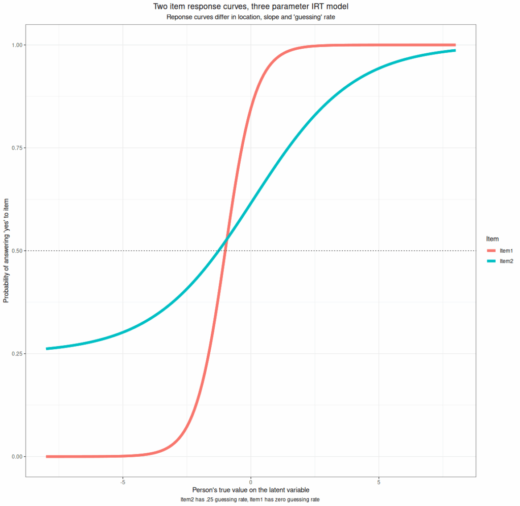
- Three parameter models. These add a parameter that allows “guessing”, i.e. that if the respondent has no preferred answer they won’t omit the item but will just give a random answer. This makes sense in knowledge testing MCQs (Multiple Choice Questionnaires) though less so if those are scored penalising incorrect answers. They don’t really make sense for our measures. Here is an example nevertheless.
Caveat 1: multiple IRT models for short ordinal responses #
This is a rather sad little caveat but it has generally discouraged me from using IRT models: there are different ways of handling the estimation of the response curves for the cutting points in short ordinal response curves and I have found that they can give rather different findings and I don’t really understand the differences!
Caveat 2: (the big one) “local stochastic independence” #
I used to find the IRT model seemed attractive as the assumption of interval scaling in CTT seemed implausible. However, the one crucial requirement for estimation of the Mokken characteristics of a measure to be possible is that all the items of the measure “are locally stochastically independent”. This is essentially saying that the likelihoods of any pair of items being answered positively is only affected by the latent variable and not by any other aspect of the participants or the items, i.e. the items must be pure measures of the latent trait and uncontaminated by any other source of variance. I can see that this is necessary for the maths of Mokken scaling (and any IRT model I think) to work but it’s very unlikely to be true for any measure in our areas. This in no way invalidates using Mokken scaling or other IRT: they are clearly very useful if your measure is not far off undimensional (or if the items you analyse from it are nearing unidimensional) and if contributions to responding from other variables are small (which pretty much says the same thing in different words). When invalidating variance and deviations from unidimensinality are small then these methods can really help us explore how plausible the mapping of responses to scores looks. However, for me this is rather like seeing how implausible the assumptions of CTT look: IRT of all types is dependent on another set of assumptions, amounting to this “local stochastic independence” which are just as necessary for IRT to work as the assumptions of CTT are for it to work but all these assumptions are never going to fit perfectly for our measures and the realities of measuring change in psychosocial interventions. We need to use them with humility rather than hubristic excitement about their apparent power to give us precise measurement of things that are never directly measurable.
Try also #
- Classical Test Theory (CTT)
- Mokken scaling
- Psychometrics
- Rasch model
- Reliability
- Unidimensionality
- Validity
Chapters #
Not covered in the OMbook.
Online resources #
None likely.
Dates #
First created 11.v.25, links tweaked to add Rasch moldel 14.v.25.

