A term that used to be used a lot in reporting psychometric explorations of self-report questionnaire data which is so common in our field. However, the term is being used less and less as factor analysis of the correlations between item scores moves from using almost exclusively exploratory factor analysis (EFA) to almost entirely confirmatory factor analysis (CFA). In CFA the factor structure is specified in the analysis and the software returns a lot of diagnostic information about how closely the empirical data appear to fit that structure (hence “confirmatory” though the adjective often implies much more strength to the findings that is really the case when one looks closely at what has been done).
Details #
So what does the term mean? The principles are the same in CFA and EFA but what you get is rather different.
CFA #
In CFA it is what you think applies in mapping observed variables (item scores) to presumed underlying factors (“latent variables”, “common factors”). Using whatever syntax your CFA software expects, you tell this to the software. To use my favourite measure for these examples, the HADS (Hospital Anxiety and Depression Scales). The desired factor structure is for all the seven anxiety items to load (correlate with) a single factor and all seven depression items to load on another common factor and it sensible to assume that this is an “oblique structure”: that the those two factors correlate with each other. To mop up the any variance that can’t be accounted for by those mappings it is also assumed that each item has its own “error” or “unique” variance: variance that is not down to those two factors. The final assumption in that factor structure, or model of the functioning of the measure, is that the 14 error variances are not correlated with any other error variance nor with the the two “common” factors. A CFA analysis will give a set of measures of misfit and a set of “modification indices”: additional loadings that would improve the fit. These are typically correlations between those “error” or “unique” variances or “cross-loadings”: mappings between an anxiety item and the common depression factor (or vice versa). Here is that mapping in Lavaan syntax (Lavaan is one of the packages doing latent variable analyses in R).
HADSmodel <- 'Anx =~ HADS01 + HADS04 + HADS05 + HADS08 + HADS09 + HADS11 + HADS13
              Dep =~ HADS02 + HADS03 + HADS06 + HADS07 + HADS10 + HADS12 + HADS14
              Anx ~~ Dep'
That is saying that a factor “Anx” underlies variation on items 1, 4, 5, 8, 9, 11 and 13 of the HADS, that another factor, “Dep” underlines variation on the other items (2, 3, 6, 7, 10, 12, and 14) and the last line says that the two factors may be correlated with each other. That gives us this factor structure as a set of loadings (and some other information).
Latent Variables:
                   Estimate  Std.Err  z-value  P(>|z|)
  Anx =~
    HADS01            0.526    0.036   14.641    0.000
    HADS04            0.224    0.032    6.957    0.000
    HADS05            0.635    0.043   14.922    0.000
    HADS08            0.424    0.036   11.850    0.000
    HADS09            0.378    0.037   10.191    0.000
    HADS11            0.428    0.042   10.215    0.000
    HADS13            0.630    0.040   15.937    0.000
  Dep =~
    HADS02            0.377    0.033   11.264    0.000
    HADS03            0.629    0.044   14.336    0.000
    HADS06            0.387    0.030   13.111    0.000
    HADS07            0.450    0.032   14.278    0.000
    HADS10            0.320    0.042    7.622    0.000
    HADS12            0.386    0.032   12.079    0.000
    HADS14            0.313    0.040    7.906    0.000

Covariances:
                   Estimate  Std.Err  z-value  P(>|z|)
  Anx ~~
    Dep               0.919    0.025   37.371    0.000

Variances:
                   Estimate  Std.Err  z-value  P(>|z|)
   .HADS01            0.344    0.027   12.635    0.000
   .HADS04            0.358    0.025   14.360    0.000
   .HADS05            0.475    0.038   12.518    0.000
   .HADS08            0.388    0.029   13.526    0.000
   .HADS09            0.441    0.032   13.887    0.000
   .HADS11            0.562    0.040   13.883    0.000
   .HADS13            0.386    0.032   12.034    0.000
   .HADS02            0.342    0.025   13.578    0.000
   .HADS03            0.513    0.041   12.572    0.000
   .HADS06            0.247    0.019   13.041    0.000
   .HADS07            0.265    0.021   12.597    0.000
   .HADS10            0.599    0.042   14.249    0.000
   .HADS12            0.302    0.023   13.363    0.000
   .HADS14            0.526    0.037   14.211    0.000
    Anx               1.000
    Dep               1.000
The first block there tells us the loadings for each of the items allowed to load (have responses driven by) on the presumed common factors. The first set are the anxiety items, the next are the depression items. All the loadings (labelled “Estimate” as these are estimates of population loadings) are highly unlikely to have arisen by chance as indicated by the p values (derived from the standard error and z values but we’ll skip that here!)
Then the output gives the covariance between the two common factors. As their variances have been set to 1.0 (a so-called “standardised” solution) the covariance is also the correlation. It is very high at .919 and this estimate won’t have arisen by chance sampling from an infinite population in which the covariance is zero. (This is all using the NHST, Null Hypothesis Significance Testing paradigm.)
The final block give the error variances for each item, again, they are all statistically significant: very unlikely to have arisen by random sampling from an infinite population in which their variances are zero, i.e. in which all the variance on the items was caused by the common factor for that item.
A nice way to look at such loading matrices is a path diagram. From analysing these HADS data the path diagram looks like this.
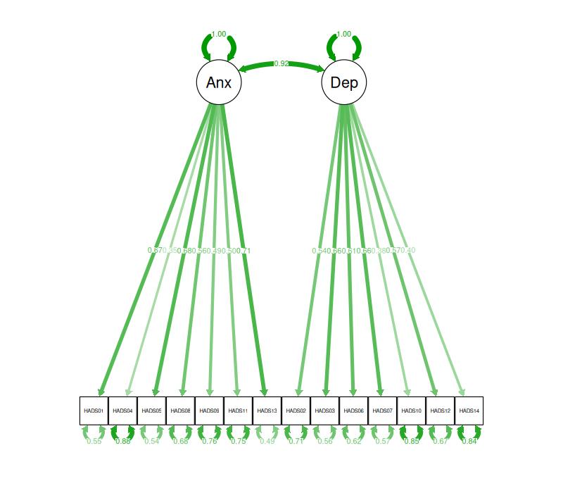
[Sometime soon I must create an entry about path diagrams and link to it here!]
So that is the factor structures of the HADS as estimated by CFA for this dataset first as formula that specified the CFA, then as a loading matrix and finally in a plot (with the estimated values for the various parameters in the model).
EFA #
In EFA you would tell the computer program to report loadings for just two common factors (in principle it can extract 13) and a correlation between those two factors and you would look to see if the anxiety items load clearly more strongly on one common factor and the depression items loading more strongly on the other factor. The program would give you a correlation between the factors (with various different ways of choosing that) and would again give uniquenesses (though in EFA these are flagged more by an overall opposite of the uniqueness: the “commonalities” of each factor.
Here is a the factor structure of the same data obtained by EFA. I specified extraction of just two factors and asked for an oblique solution (i.e. potentially correlated factors).
Standardized loadings: (* = significant at 1% level)

            f1      f2       unique.var   communalities
AH01anx      .   0.566*           0.571           0.429
DH02dep  0.601*                   0.618           0.382
D03dep           0.746*           0.444           0.556
AH04anx  0.579*                   0.719           0.281
AH05anx          0.775*           0.451           0.549
DH06dep  0.594*      .            0.557           0.443
DH07dep  0.393*  0.335*           0.583           0.417
AH08anx      .*  0.352*           0.684           0.316
AH09anx          0.520*           0.735           0.265
DH10dep  0.442*                   0.806           0.194
AH11anx          0.433*           0.764           0.236
DH12dep  0.728*                   0.506           0.494
AH13anx          0.751*           0.440           0.560
DH14dep  0.380*                   0.820           0.180

                              f2    f1 total
Sum of sq (obliq) loadings 2.941 2.360 5.301
Proportion of total        0.555 0.445 1.000
Proportion var             0.210 0.169 0.379
Cumulative var             0.210 0.379 0.379

Factor correlations: (* = significant at 1% level)

       f1      f2
f1  1.000
f2  0.574*  1.000
Here again the first block, the loading matrix, gives the estimated loadings of the items on the common factors. Instead of giving SE, z and p values this lavaan output simply flags the loadings that were unlikely to have arisen by chance at p < .01 with asterixes. The blanks are where the loading was below an arbitrary (but commonly used) criterion of .4. The last two columns give two versions of the same thing: how much of the variance on the item in the dataset is down to the loadings on the common factors, the uniqueness values are the complement of this: the proportion of variance on the item that is not down to the common factors.
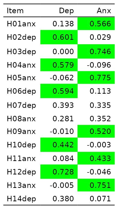
There is a weak cross loading for item 8 on depression too although the loading is clearly smaller than .4 as that cell in the loading matrix has been blanked out. Here is the same two factor loading matrix formatted differently with green highlighting on the loadings greater than .4.
And here is the same as a path diagram. (I’ve renamed the items to overcome the way that the plot software chopped the “anx” and “dep” off!)
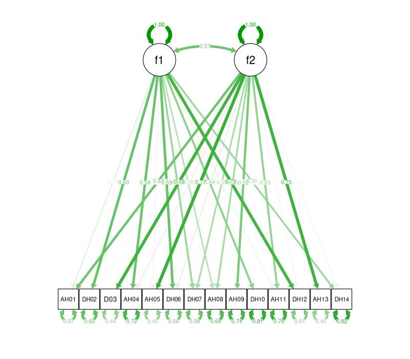
As factor analysis was always EFA before the computational power the algorithms for CFA came along “factor structure” used to mean pretty much this matrix. Here you can see a fairly “clean” structure as each item loads more strongly on the factor it was designed to reflect. However, item 7 shows “cross loading”: it has strong loadings on both factors. Cross loading will only show up in CFA in “modification indices” (MIs)which show where allowing a loading initially disallowed in the CFA model would improve overall fit. Interestingly, the MI for item 7 loading on the anxiety factor was 2.2 suggesting that allowing this cross-loading in the CFA would improve fit (values above 2 tend to suggest that will be the case). However, the values of other MIs in the CFA model are vastly larger with an MI of 106 for allowing a loading of the anxiety factor onto item 3. This illustrates that EFA and CFA can show rather different things.
Other terms you used to see describing factor structure in EFA were “low/negligible loadings” when the loadings of an item on any common factor were all small (typically defined as below .4 though sometimes smaller criteria were used. The other term was “incorrect” or “mismapped” loading when an item loaded on a common factor that it wasn’t designed to measure and didn’t load meaningfully on the factor it was supposed to reflect.
Summary #
So either way, EFA or CFA, “factor structure” tells you, for the data and measure being reported, how well the data appear to fit the design intentions for the measure.
Try also #
- Confirmatory Factor Analysis
- Construct validity
- Exploratory Factor Analysis
- Factor analysis
- NHST paradigm
- Psychometrics
- Scree plot
Chapters #
Not covered in the OMbook.
Online resources #
I can see that I really need to do an Rblog and perhaps some additions to this and related factor analysis definitions here. I will try to find time soonish!
Dates #
First created 7.iii.26, updated adding HADS CFA 9.iii.26 and EFA 12.iii.26, link tweak 30.iii.26.

