I think it’s pretty unlikely that you will come across this term reading research reports in our field but this process underlies so much statistical computation used in our field that I think it’s probably useful to know about it.
Details #
As computers are digital, that is to say they actually don’t handle continuous numbers but with lumpy, discontinuous numbers that can be expressed as sums of powers of 2 (as they are basically binary machines). This means that they don’t solve problems by solving equations, generally they solve problems by methods of approximation. As a very simple example, say you want the square root of a number. One method of approximation is to say that the answer must be somewhere between that number and 1 (as we know that the square root of a number is the number that, multiplied by itself is the number. So
where the symbol “\(\sqrt{}\)” represents “square root” in usual algebra or:
sqrt(9)*sqrt(9) == 9
In typical R code.
So a first approximation to \(\sqrt{9}\) might be 4.5 as that’s halfway between 0 and 9. (Yes, I know you know that \(\sqrt{9}\) is 3 but I bet you don’t know to five decimal places what \(\sqrt{47}\) is, I’m use \(\sqrt{9}\) for illustration!!)
OK, but 4.5*4.5 is 20.5 so 4.5 is clearly too big so now let’s try 4, that gives us 16: still too big. We could blunder on like this but there is a good method to guide iteration:
this will always converge toward the accurate value of \(\sqrt{9}\) if the first guess (i.e. the starting approximation) is a real number. Here’s what we get if we start from 4.5

So that gets to the correct answer in six iterations after that first bad guess.
This method is very computationally efficient and was probably known to Babylonian mathematicians. The principle is that you stop iterating as soon as the change from the last approximation to the current one is small enough for your needs. Here’s that as a plot.
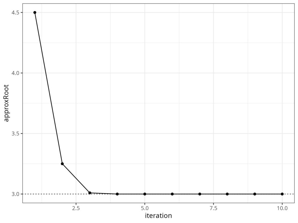
The dotted line marks the correct answer: 3.
This is not how any modern software running on any modern hardware would do this but it conveys the principle that many modern statistical analyses of even mildly complex models will use methods of “numerical approximation” to reach their answers and they will use a stopping criterion to give a very high degree of precision for all the numbers in the findings, a far high precision than we ever need in our field. Most modern statistical analyses will look at multivariate data and the answers/findings often involve many numbers, see e.g. confirmatory factor analysis or principal component analysis. The approximation method above, the Babylonian or Heron’s method is specific to finding square roots. (Heron was a Greek mathematician who discovered it probably without knowing that the Babylonians had already found it.) However, there are now many, many methods of approximation that exist as computer algorithms and it’s a huge area of applied maths and of statistics knowing which methods are best for what questions and “best” can mean “faster”/”less computationally expensive” and/or “robust”, i.e. likely to reach the correct answer. (See “local minima” for one issue here and a useful metaphor for quite a lot of trying to find answers to complex questions quite outside of numbers and stats.) Approximation methods can be very sensitive to the starting guess, if you give the Babylonian method the starting value of -4.5, it converges on -3 which is a square root of 9 (as -3*-3 = 9) but it might not have been the answer you expected.
Try also #
- Approximation (general)
- Confirmatory factor analysis (CFA)
- Local minima
- Principal component analysis (PCA)
Chapters #
Not covered in the OMbook.
Online resources #
None currently or likely I think.
Dates #
First created 21-22.iii.26.

