Path diagrams

I am someone who loves to see data: tables are lovely and I think, having been at it for at least forty years now, I can say that I am not bad at reading them. However, I love to see a good visualisation of data so I was bound to be a sucker for path diagrams. They what they say: they visualise “paths”. They don’t have to have any numbers in them but often do.

Details #

So what’s a “path”? It’s a presumed influence from one variable to another. The first important thing to know about path diagrams is that the variables may be measured or “latent” i.e. unmeasured and potentially unmeasurable. Here is a very simple path diagram.

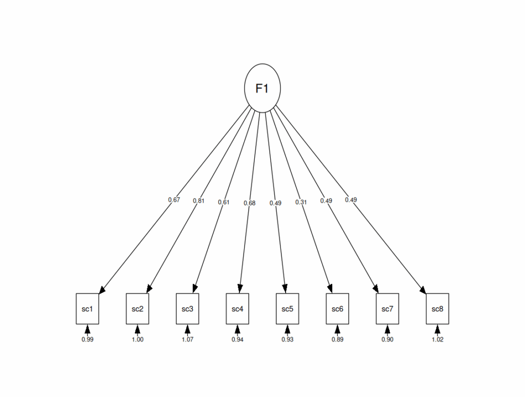
That shows a single factor model with eight measured variables: sc1 to sc8 (“sc” for score, this is a typical model of an eight item questionnaire measuring some presumed underlying variable: “F1” (for “Factor 1”). That is not directly measurable: as so often in our areas we measure it indirectly by assuming that it is influencing answers on all the measured variables: the questionnaire items.

The convention in path diagrams is that measured variables are indicated by squares and latent, unmeasurable, variables by circles and the paths are the lines.

But what are these “paths” these influences? The crucial thing to understand is that these are not about what is going on for individuals but about associations across all the responses on the eight items from all the participants contributing to the dataset. This is a simulation with 500 simulated participants and the assumption is that there is some shared tendency and that across the 500 participants some have more of this “latent”. Let’s say here it’s data from a survey of 500 therapists and the eight items are asking about how much they think they use observations of visible reflections of stress in their clients. Then the factor model assumes that some of the 500 think they use these cues much more than others do. Of course, if that model is true then there will be a tendency for one individual to respond differently from another but these lines are not like a snooker cue hitting the items to create responses, the levels of the differences between the therapists may actually be quite small but across 500 they may create a clear pattern of correlations in scores on the items that can by pushing the 4,000 (8 x 500) item responses through a factor analysis which gives this table.

Latent Variables:
Estimate Std.Err z-value P(>|z|)
F1 =~
score1 0.666 0.058 11.508 0.000
score2 0.806 0.061 13.171 0.000
score3 0.606 0.059 10.330 0.000
score4 0.680 0.057 11.929 0.000
score5 0.493 0.054  9.195 0.000
score6 0.309 0.051  6.115 0.000
score7 0.491 0.053  9.281 0.000
score8 0.494 0.056  8.855 0.000

Variances:
Estimate Std.Err z-value P(>|z|)
.score1 0.986 0.074 13.243 0.000
.score2 1.001 0.083 12.098 0.000
.score3 1.067 0.077 13.854 0.000
.score4 0.935 0.072 12.988 0.000
.score5 0.929 0.065 14.326 0.000
.score6 0.892 0.059 15.207 0.000
.score7 0.903 0.063 14.294 0.000
.score8 1.018 0.070 14.450 0.000

F1 1.000

That’s pasting the output form a cfa() function analysis of my simulated data. cfa() is a confirmatory factor analysis function from the brilliant R lavaan package. There is a lot of information there. The red block gives the paths from the latent factor to the items. The blue block gives the “residuals” or “error” terms, another set of unmeasured variables, one per item representing the variance across the 500 completions of each item that is not explained by the path from the latent variable. those are shown here by little paths onto each of the observed variables. The final black bit just says that I had asked for the cfa() function to find a solution with the variance of the latent variable set to 1.0. (Long story, not for here!)

If you look back up to the path diagram you can see that the first column of the red block has been shown on the paths from the latent to the observed items and you can see that the first column of the blue block are shown below the observed item variables.

A slightly more complex path diagram #

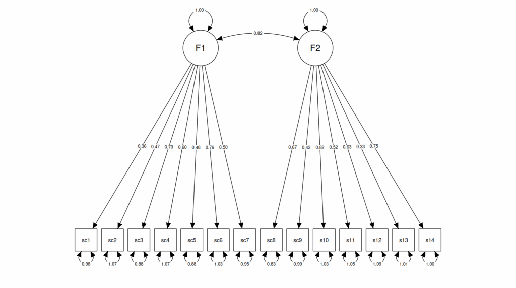
That shows a two factor as opposed to a single factor path diagram and introduces the last two symbol you need to understand most basic path diagrams: the curved, two-headed arrow to represent a correlation which is shown for the correlation here between the two separate latent variables. A looped, two-headed arrow is also introduced here to mark the variances of the two latent factors and the variances of the errors in measuring the observed variables.

The basic path diagram symbols #

• Square = measured/observed variable
• Circle = uneasurable/latent variable
• Single-headed arrow = a “path”, a unidirectional effect
• Curved two-headed arrow = a correlation
• Either a stub single-headed arrow (first figure above) or a looped two-headed arrow two and from the same variable (second figure above) can be used to represent a variance of an effect

summary #

This had to take us quite deeply into factor analysis, here a confirmatory factor analysis. Path diagrams can be used for many other models including linear regressions and more complicated models. There are also different conventions about how exactly path diagrams should be drawn but the basics of the lines, the square measured variables and the circles for the unmeasurable variables are consistent. Anyway, I hope this introduction has shown enough to show how useful they can be.

Try also #

• Confirmatory factor analysis
• Covariance
• Covariance structure models
• Exploratory factor analysis
• Factor analysis
• Latent variable models
• Linear regression
• Variance: introduction
• Variance: computation and bias

Chapters #

Not covered in the OMbook.

Online resources #

May be more in the Rblog in the future.

Dates #

First created 26.iv.25, updated with two factor diagram and list of symbols 29.iv.25.