Computer intensive statistical methods mainly used to obtain robust estimates of confidence intervals around observed sample statistics though they can also be used to get statistical signficance tests: p values.
Details #
[This and the jackknife method explanation start from the same scenario.]
Scores on a measure from 880 participants look like this.
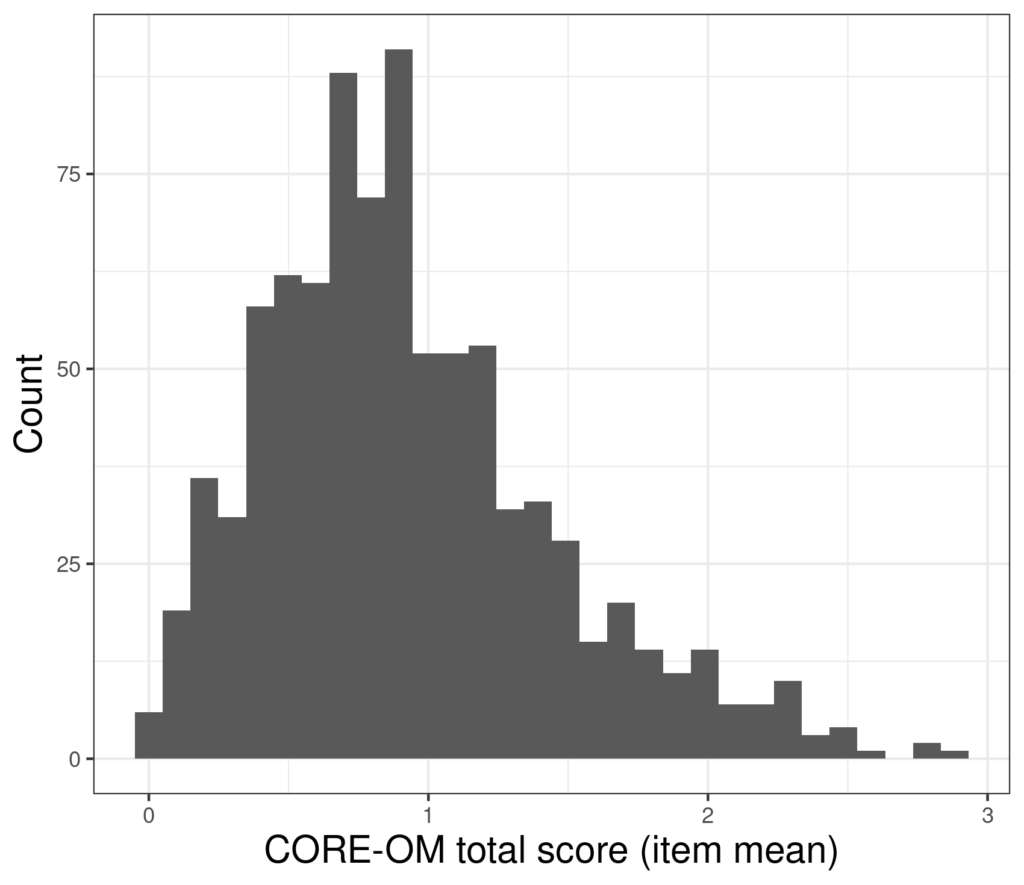
The mean of those scores is .93 and the standard deviation is .52 so the parametric standard error of mean (which is SD/sqrt(n)) is .52/sqrt(880) = .52/29.7 = 0.018 so the 95% confidence interval around our observed mean +/- 1.96 * 0.018, i.e. from .90 to .97.
However, the problem is that that calculation is “parametric”: based on the assumption that the distribution of the data is Gaussian and completely defined by two population parameters (hence “parametric”): the mean and the SD. (This is also sometimes expressed as being defined by the mean and the variance but as the SD is square root of the variance, that’s saying the same thing: that we are working from the assumption that the distribution is Gaussian and that therefore it is completely defined by just two parameters.) However, using a parametric method means that the estimate of the CI of the statistic, here the mean, will be poor if the distribution of the data isn’t Gaussian. Looking at that histogram shows that these data are incredibly unlikely to have come from a Gaussian population. They have a finite range not an infinite one, they actually only take discrete values (neither of those issue are terribly problematical for most parametric methods) but crucially the distribution is clearly positively skew: with a longer tail to the right than the left.
Bootstrap estimation gives a CI that is (almost always) robust to the distribution of the data. The process involves “resampling”: creating a new sample of n = 880 by sampling “with replacement” from the actual 880 observed values and computing the mean for that resample, and doing this again and again. “With replacement” means that any observation may occur in the resampled data set any number of times: zero, once, twice, even theoretically 880 times (but the probability of that happening is so low it can be ignored in the likely life expectancy of our planet or perhaps our universe). Doing this repeatedly creates a set of computed means and that distribution is used to get the confidence interval around the observed statistic, here the mean.
You can see why this is one of the “computer intensive” methods: that’s a lot of computing. However, modern hardware does this sort of thing in a flash.
If the replications are created truly randomly, different runs will give different data. However, the larger the number of times you create these “bootstrap replications” the more stable your answer.
Here are the means from 10,000 bootstrap resamples from the data above.
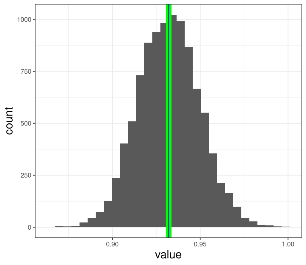
Here the mean of those estimates is shown by the green line and the observed sample mean in blue and they are clearly almost identical (but unlike the jackknife method, the mean of the replications is not guaranteed to be exactly the same as the observed sample mean). Those values range from .865 to .998. We can see that this is computer intensive: generating 10,000 means of 880 resampled values took .6 of a second on my three year old, but fairly powerful, laptop.
There are actually a number of different ways to get the confidence interval from that distribution. In reports the ones you are likely to see are “simple/basic”, “BCA” (Bias Corrected and Accelerated), “Normal” and “Percentile”. There are a few others but they are essentially esoteric for us. Here are the 95% CIs for the mean from this bootstrapping of these data.
| Method | LCL | UCL |
| Basic | .897 | .966 |
| Normal | .898 | .967 |
| Percentile | .899 | .967 |
| BCA | .899 | .967 |
Effect of sample size #
Of course, any confidence interval around any observed statistic will be wider the smaller the sample. As in the example for the jackknife method, here are the scores from a reduced sample of n = 44.
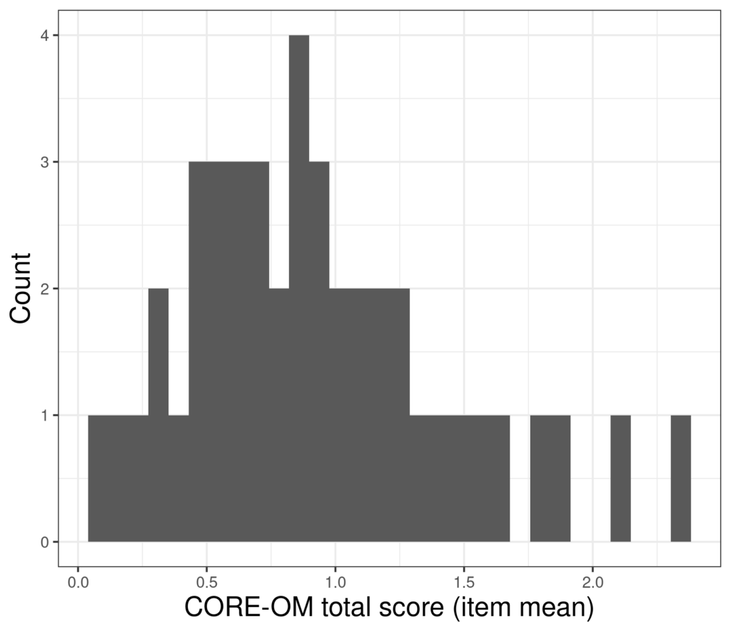
And here are 10,000 bootstrap resampled mean from that smaller dataset.
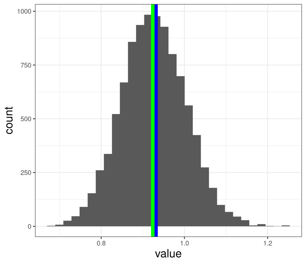
Here we can see that the mean of the bootstrapped data (green, .926) is not exactly the same as the observed sample mean (blue, .928) and these means range from .682 to 1.24, a much wider range than that (.865 to .998) we had from the full sample of n = 880. Here are the 95% confidence intervals from this sample.
| Method | LCL | UCL |
| Basic | .775 | 1.08 |
| Normal | .777 | 1.08 |
| Percentile | .779 | 1.08 |
| BCA | .787 | 1.09 |
Of course, these are considerably wider than those from the full sample.
Setting the rnG “seed” to get the same answer every time #
Because the resampling is random you can get slightly different bootstrap derived confidence intervals around your observed statistic every time you generate your resamples. The way computers generate numbers is a sophisticated area of maths and programming but most RNGs (Random Number Generators: the algorithms used by the computer) use a “seed”. If you set the same seed before running your bootstrap you will get the same CI every time.
Summary #
There are some subtleties being left out here but this is a fair, and fairly comprehensive, introduction to the method. When bootstrap methods are used in a research paper the methods section of the paper should state the software used, the number of bootstrap resamples and what method of determining the CI and how many resamples were computed.
Try also #
Jackknife method
Distribution
Parametric statistics
Estimation
Precision
Sample
Population
Mean
Variance
Standard Deviation (SD)
Chapters #
Not mentioned in the book but methods used in the examples in chapter 8.
Dates #
Created 13/11/21, text improved a bit and issue of setting the RNG seed added 14.i.v26.

