The earliest of the computer intensive statistical methods. (I think it’s almost always written “jackknife” but I have put “jack-knife” in case, like me, people sometimes put the hyphen in.)
Details #
[This and the bootstrap method explanation start from the same scenario.]
Let’s take the simple example: suppose we want to know the 95% confidence interval (CI) of the mean of a set of scores on a measure and the distribution of the 880 scores we have looks like this.
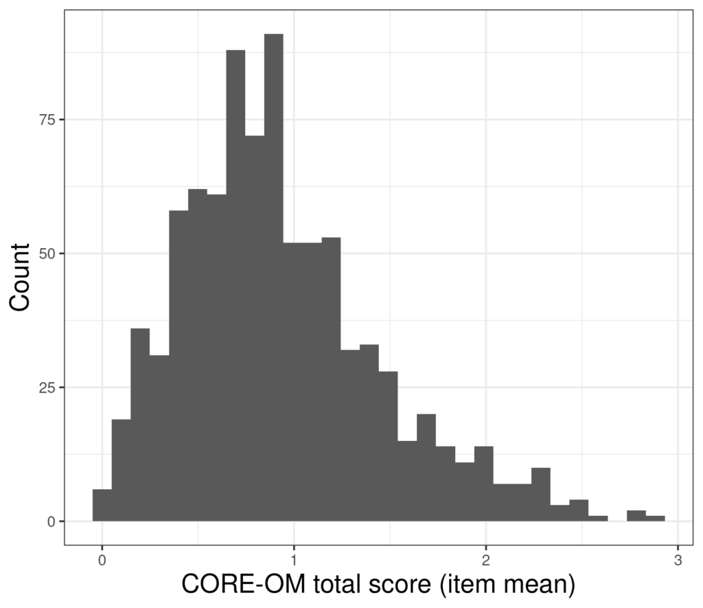
The mean of those scores is .93 and the standard deviation is .52 so the parametric standard error of mean (which is SD/sqrt(n)) is .52/sqrt(880) = .52/29.7 = 0.018 so the 95% confidence interval around our observed mean +/- 1.96 * 0.018, i.e. from .90 to .97.
However, the problem is that that calculation is “parametric”: based on the assumption that the distribution of the data is Gaussian and completely defined by two population parameters (hence “parametric”): the mean and the SD. (This is also sometimes expressed as being defined by the mean and the variance but as the SD is square root of the variance, that’s saying the same thing: that we are working from the assumption that the distribution is Gaussian and that therefore it is completely defined by just two parameters.) However, using a parametric method means that the estimate of the CI of the statistic, here the mean, will be poor if the distribution of the data isn’t Gaussian. Looking at that histogram shows that these data are incredibly unlikely to have come from a Gaussian population. They have a finite range not an infinite one, they actually only take discrete values (neither of those issue are terribly problematical for most parametric methods) but crucially the distribution is clearly positively skew: with a longer tail to the right than the left.
The jackknife method estimates the standard error by looking at the distribution of means of the data leaving out one observation at at time. So we have 880 observations, the first “jackknife” estimate is the mean of observations 2 to 880, i.e. leaving out the first observation, the second estimate is the mean of observations 1 and 3 to 880, and so on until the last estimate is the mean of observations 1 to 880.
Here’s are those estimates.
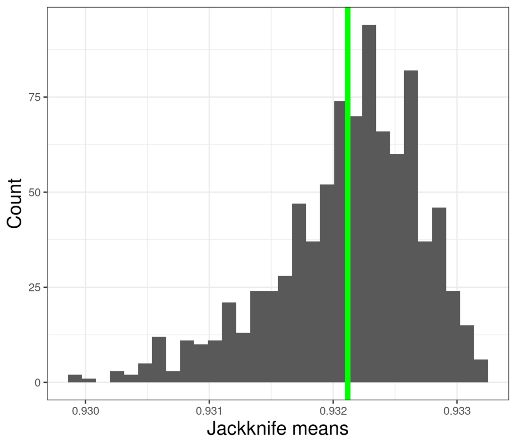
So these the 880 jackknife estimates of the sample mean. We can see that they have a fairly tight range, actually from 0.9298995 to 0.9331786. The green line is their mean and that’s always the same as the sample mean. What is useful is that the distribution of these values gives us a “robust” estimate of the variance of the mean and a robust 95% CI for that mean based on the variance of these estimates. (“Robust” means that the estimate is not based on an assumption of Gaussian distribution that is clearly violated, it is robust to deviation from Gaussian.)
For these data this jackknife 95% CI is from .898 to .967. Here the answer is the same as the parametric estimate (.897 to .966) to 2 decimal places but we have the reassurance that it is “robust”, where the distribution of data deviates much more markedly from Gaussian the parametric and jackknife CIs will deviate more markedly and the parametric estimate will be tighter than it should be and may also be biased, i.e. not centred correctly.
However, gaining this robustness was computer intensive: it involved computing 880 means of 879 values. That’s not particularly challenging even for early computers and for small datasets it can be done with a mechanical calculator. The method was invented in 1949 when computer power was still very limited and things often done by hand.
Effect of sample size #
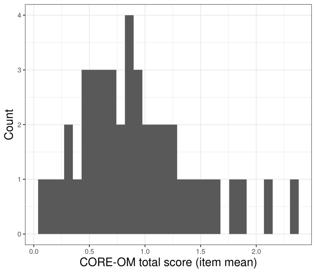
We can see that the jackknife must have the correct property of much lower variance in those estimates in large samples. To show that I took just 44 evenly spaced scores from the 880 so the raw sample data now look like this:
Now the jackknife estimates of the mean look like this.
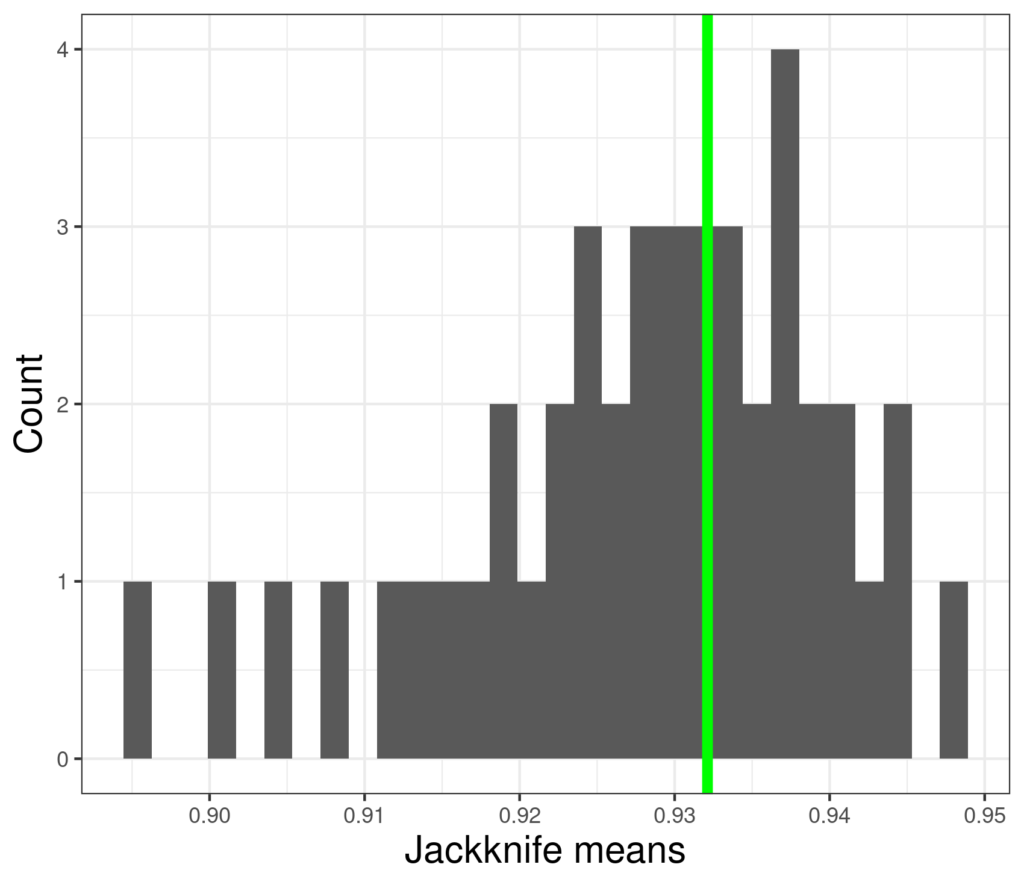
These means range from 0.8945198 to 0.9471873: much wider than the range for the full dataset of 880 values and the 95% CI is now from .771 to 1.084 (the parametric CI was .775 to 1.080, again the same as the jackknife to 2 decimal places).
Summary #
The jackknife method can be applied to many sample statistics, not just the mean. However, it has been almost completely replaced by the bootstrap method.
Try also #
Bootstrap methods
Computer intensive methods
Distribution
Estimation
Parametric statistics/tests
Precision
Sample
Population
Mean
Variance
Standard Deviation (SD)
Chapters #
Not mentioned in the book but methods used in the examples in chapter 8.
Dates #
Created 13.xi.21, tweaks 15.iv.26.

