In psychoanalytic/psychodynamic theory when one slips into an chronologically, developmentally earlier way of functioning as when I get very childish when some aspect of IT fails to work for me as I think it should. Hm, actually not that as that’s not really me in the grip of unconscious processes: psychological processes that I cannot, despite wanting to, pull into conscious inspection.
No, what this entry is about is the algebraic arena of linear regression and the statistical arena of linear regression analyses. A lot of this overlaps with the entry about Linear versus non-linear processes/relationships but this gives an introduction to linear regression analyses as statistical methods.
Details #
All linear relationships have an equation of the form:
\(y=mx + c\)
And they always plot in scatterplots as straight lines:
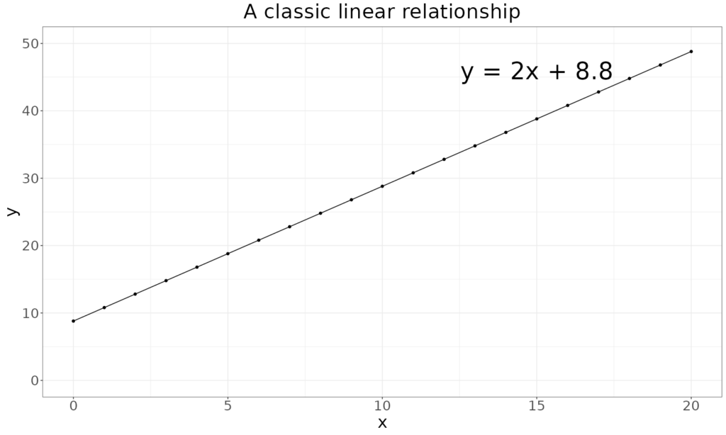
The equation says that the y value, here perhaps a well-being score, is made up of some multiple, m, of the x value and a constant, c. So in that plot c is 8.8 and m is 2. Linear functions can also be functions of more than one predictor:
$$y = mx + nz + c$$
In real life as opposed to nice linear algebra, things are messier, like this:
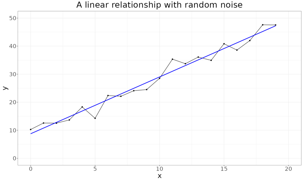
The statistical method of linear regression assumes that we have a relationship like this:
\(y=mx + c + \text{error}\)
The assumption is that the systematic relationship between the y variable and the x variable is linear with an “offset”: the value where the straight line intersects the y axis, 8.8 in the first plot above. The further assumption is that random error, noise, is superimposed on that relationship. Linear regression analysis applies a few other assumptions. Simplifying a little the assumptions are as follows.
* That the observations are independent (which would be true if those were well-being scores of 21 different individuals at the end of their therapies who happened to have stayed in therapy for zero sessions (just an assessment meeting), one session, two sessions … and through to someone who stayed for twenty sessions but would not be true if these were all observations from one person at assessment and each session through to session 20.
* That the x values are measured accurately (technically with no measurement unreliability).
* That the variance of the y variable is constant across the range of the x values (“homoscedasticity”).
* That the population distribution of the variables of the error is Gaussian (“Normal”).
* That the error is uncorrelated with x or y.
If this model fits the real data then linear regression analysis will be able to find the best fitting straight line that satisfies that linear regression model equation above.
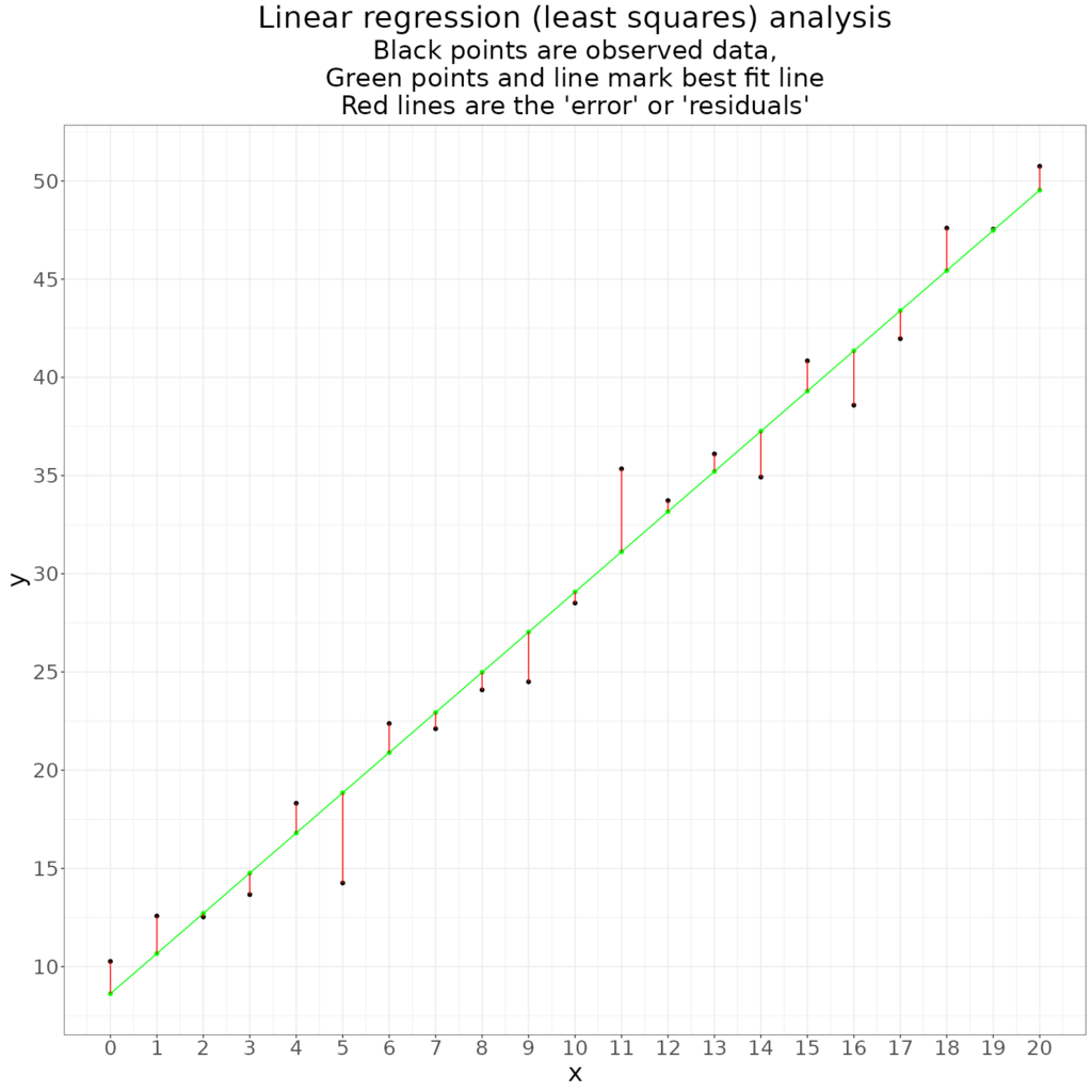
The maths of the analysis found the best fitting line by minimising the total error: minimising the total of the squares of the lengths of those red lines. (Hence this is also called “least squares regression”. The squares are used not the raw lengths as, for the best fit, the lengths will sum to zero: the total length of the ones above the fitted line exactly matching the total length of the ones below the line.)
The maths give us the intercept, c, which here was 8.6, and the slope, m, 2.05. We know, as I simulated the data, that the “true” equation of the values before I added noise was:
$$y=2x+8.8$$
so we can see that with only 21 data points and not too much noise the analysis has fitted a line very close to the perfect one had there been an infinite number of points. (The population from which our 21 points are a sample.)
The analysis also tells us how likely it is that those values of m and c would have each been as far from zero given the sample size and data had the true population values been zero, i.e. had there been no linear relationship between x and y and a mean y value of zero. For our data the answer is that it is vanishingly unlikely that we would have seen m and c as far or further from zero as the values we did see (2.05 and 8.6) given that “null model” of no linear relationship. This is typically show in an table like this:
Coefficients:
            Estimate Std. Error t value Pr(>|t|)
(Intercept)  8.61813    0.88540   9.734 8.12e-09 ***
x            2.04569    0.07574  27.010  < 2e-16 ***
---
Signif. codes:  0 ‘***’ 0.001 ‘**’ 0.01 ‘*’ 0.05 ‘.’ 0.1 ‘ ’ 1
That rather dense table tells us that c here shown to five decimal places as 8.61813, had a probability of having appeared this big or bigger (as an absolute number, minus 8.61813 would have been equally unlikely) given the null model of 0.00000000812 which is one in 123,152,709: not very likely! Similarly, the probability of a value of m as high as or higher than 2.04569 was so small that it’s actually dropping below the precision of the computer to represent it accurately but it’s lower than 0.0000000000000002.
That’s all in the traditional NHST (Null Hypothesis Significance Testing) statistical paradigm. A more sensible way of looking at this is to get the 95% confidence interval around the fitted line. That is shown here.
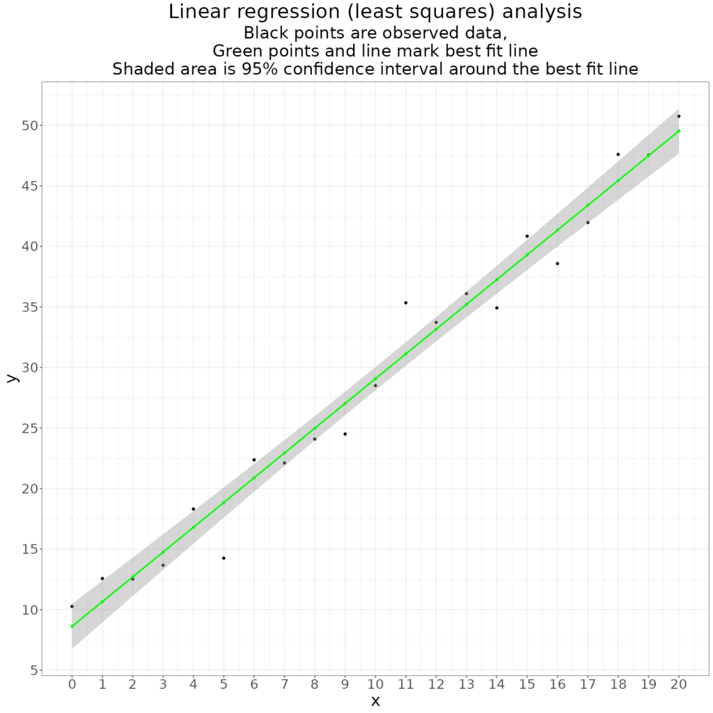
We can see that the line is estimated pretty precisely. Linear regression, if the data fit the model fairly well, always shows tighter estimation nearer the mean of the data.
Try also #
Confidence intervals
Modelling
Null hypothesis significance testing
Power relationships (mathematical/statistical)
Transforms/transforming data
Chapters #
Doesn’t feature in any of the chapters though the analyses mentioned in Chapters 7 and 8 use related methods.
Online resources #
None specifically
Dates #
First created 21.xii.23

