Historically one of the paradigmatic, genuinely paradigm changing, statistical “tests”. It tests how likely it is, given the two sets of values, that the difference between their means is so large, in the light of the variance of each set, and the sizes of the sets, that we should reject the hypothesis that they came from populations in which the means were the same, i.e. that the mean difference was “statistically significant”
Details #
I thought it would be easy just to point you off to a good web page that explains the details, certainly if you want the really detailed account then the wikipedia article is a good place to go. However, I failed to find a simpler explanations as most things I found are were about the formulae and explaining how to do the calculation. I don’t think anyone reading the OMbook or coming to this glossary needs those things: we don’t need the formulae, and only the wikipedia page tried to explain, why the formulae are as they are and these days if you need to use a t-test to analyse some data you can use a software package. I would have recommended sofastats as a free, multiplatform, open source package but I see it’s mutating (which I am sure is wise as the people who created it are impressive) … aha, the old version is still available and I’m sure it’s still robust: here.
So I have tried to give an explanation that avoids formulae and their logic and assumes that you are either trying to understand what something you have found that reports findings in terms of a t-test or that you want a bit of backgrounds before using a stats package to conduct a t-test. To be fair to the authors of the various web pages I found, I think it is actually a challenge to explain the t-test and it is very tempting to dive into formula and calculations!
There are two t-tests! #
There are actually two forms of the t-test: the “unpaired” group comparison one (which is what I described in the introduction above) and the one sample version which asks if the mean of the sample you have is unlikely to have come from a population with mean zero. That single sample version is the same as the “paired” or “repeated measures” t-test: I’ll come back to that later but the logic of the t-test is more easily explained for the single sample version.
Here is an plot of some random data.
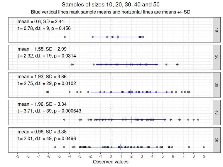
As the plot title says these are samples of sizes 10, 20, 30, 40 and 50 and the dots mark the observed values. The sample means and standard deviations are plotted in blue, vertical line for the means and horizontal for the SDs, their values are given in the labels. The labels also show the t values, degrees of freedom (“d.f.”) and the p value for the t-test with these t values and degrees of freedom.
You can see that the degrees of freedom are always one smaller than the sample size and that the formal outcome of the tests that the data came from a population with mean zero is “not significant” for the n = 10 sample (because the p value is below the conventional criterion of .05) and “significant” for the other samples. This is how the t-test works: it computes a t value and looks up (on in modern software, it computes) the p value for that t and that number of degrees of freedom. Then, following NHST logic, if that p value is less than alpha value, the risk of rejecting the null hypothesis that the population mean is zero when it really is zero, you declare your finding “statistically significant”. (By convention, the alpha value you have set before doing the test is pretty well always .05, i.e. one in twenty.)
You can also see that as the data really are random there isn’t a nice linear increase in the t values and decrease in the p values despite, as you probably guessed, the samples all coming from a population with mean 1 (and SD of 3).
This is all good in the Null Hypothesis Significance Test (NHST) paradigm. For many good reasons (see NHST paradigm and confidence intervals) it’s generally better not to use the NHST paradigm but to show the precision of estimation of the population means using confidence intervals (CIs). Here are parametric 95% CIs for the same datat
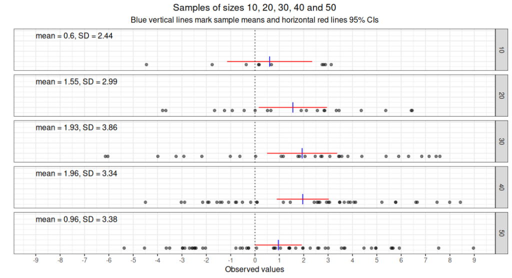
I much prefer this way of analysing most continuous valued therapy data such as measure scores.
That’s a single sample t-test, it’s the same as a paired t-test #
A paired, or repeated measures t-test is exactly the same as a one sample t-test: it just tests the null hypothesis that the mean of the differences between the first values for each participant and their later value is zero.
So what’s an “unpaired”, “between groups” oR “two sample” t-test? #
These are all names for the same thing: here you have, as the names suggest, two sets of data each independent of each other, you might be comparing the means of starting scores on some measure between two different services for example. The two groups may be very different in sizes. The formula for this t-test is somewhat different from that for the one-sample t-test: your stats package, or the report you are reading, should give you the t value, the d.f. and the p value and you compare it with your pre-chosen alpha and declare the finding statistically significant if p is below alpha, or not statistically significant if it is equal to or above your alpha.
There are always assumptions about the population for any statistical “test”: what are the assumptions for t-tests? #
Absolutely. For this classic NHST of continuous data the assumptions are:
- The observations are a random sample of an infinitely large population of such values. This is pretty much never really true of our data but it’s a sensible model.
- The observations are independent of each other: there is no “nesting” or other non-random process meaning that any one observation might be more similar to (or less) another observation. This might be untrue for our service comparison data above if one service has ten referrers referring clients from very different socioecomic settings. In that case, for that service, there is nesting and perhaps the clients from the referrer with the most deprived clientèle may have higher baseline scores for her clients than the referrer working in the most priviledged locality.
- The distribution of scores in the population (one sample t-test) or populations (unpaired t-test) are Gaussian. This is never true for our data. How much the deviation from Gaussian matters, risks invalidating our conclusions, can be quite uncertain, it can be quite serious, or trivial. This is the issue of “robustness” of the test.
- For the unpaired test, the populations are assumed to have the same variance. (Highly unlikely to be true for many of our dataset we might want to compare.)
This might mean you would see degrees of freedom that aren’t integer values. That means that Welch’s variation on the original between groups t-test has been used. That is robust (see above) to the populations having unequal variances (SDs) and is often the default that statistics packages use for between groups t-tests.
All these assumptions apply equally to computing parametric confidence intervals. However, for n >= 40 (say), you can compute bootstrap confidence intervals, that removes the need for Gaussian distributions in the population(s).
Don’t all these assumptions mean that statistical analyses are just a dark art? #
Or “Lies, damned lies and statistics” as Mark Twain, or perhaps someone else but probably not Benjamin Disraeli first said?
Not so! The problem is that over the last century in which statistical analyses have exploded into pretty much all of everyday life in the global North, we have treated them as having god like powers to divine what is right and what is wrong. They’re not, used sensibly, with awareness of their assumptions, their robustness or otherwise, they are enormously powerful and helpful ways to help us describe and interpret data. Sadly, with the advent of “machine learning”, “big data” and “AI” we are creating new false gods and ones which are much harder to understand and critique than were traditional statistical methods and their modern extensions.
Try also #
- Bootstrapping (and bootstrap methods for more explanation)
- Confidence intervals (CIs)
- NHST paradigm
- Robustness
- Welch’s test/correction
Chapters #
NHST p values and confidence intervals are covered in Chapter 5 of the OMbook.
Online resources #
None currently.
Dates #
First created 7.ii.26, updated and improved 8.ii.26, link to Welch’s test added 10.ii.26.

