
This probably doesn’t come up directly all that often in the therapy/MH literature but it underpins so much in statistics so I thought I should put it in here.
Details #
Basically it’s the distribution you expect if you do something with a binary outcome repeatedly and if the probability of the outcome you want is the same every time. Typical examples are tossing a coin wanting it to come up heads, rolling a die looking for a six or statistical tests coming up with p < .05 when in fact the null hypothesis applies. For each of those, if the process is “fair” the probabilities are 1 in 2, i.e. 1/2, i.e. 0.5; 1 in 6 = 1/6 ≃ 0.166667; and 1 in 20 = 1/20 = .05 respectively.
So if you do it just once you have a one in two chance of scoring 1 with the fair coin; a one in six chance of getting that six with the fair die and a one in twenty chance of a false positively significant result in that last (more pertinent example).
Well, actually, when you only do it once that’s not a very interesting end of the Binomial distribution, that’s also called a Bernoulli process or distribution. The Binomial includes this also covers when you do that sort of thing more than once. So the header image is a barchart of the number of sixes (i.e. score of 1) when you roll just one fair die. The bars are what happened doing that 200 times (and would be different the next time you did it 200 times: we’re talking about statistical, “stochastic” processes.
But what are the probabilities of scores of 0 (no sixes), 1 (just one six) or 2 (two sixes!) if you roll two dice? This is the binomial distribution.
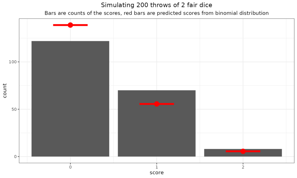
That shows the expected frequencies from the binomial distribution in red and the counts from that particular throw of two dice 200 times. (OK, as you have probably guessed, I simulated it: much quicker than actually doing it with real dice!)
We can see that even with 200 throws the fit to the predicted numbers is not perfect, that’s the reality of statistical, stochastic, random processes. What about 10,000 throws?
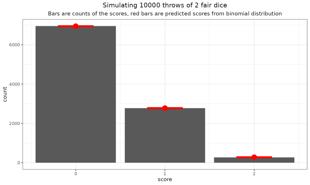
Now the fit is very good, again, that’s what you expect as you increase your sample size assuming that you are sampling randomly from an infinite number of throws and if each throw is fair, which implies independent of any of the other throws: the bigger the sample size, the better the fit to the population distribution, here the binomial distribution.
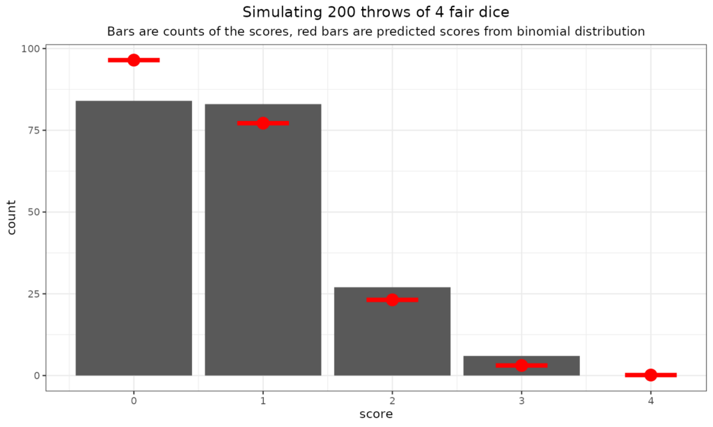
What about throwing more dice?

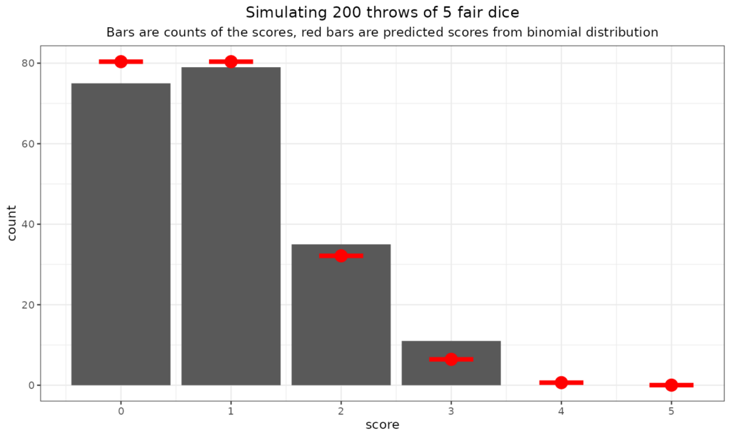
We can see that the fit to the expected rates can be perhaps less good than you would imagine with 200 throws and also that the expected rate at which you’d see three sixes is not high: one in 216 (216 = 6x6x6). It seems it didn’t happen in those 200 throws. Here we go for some more multi-dice throws (in sets of 200!)


Just to go off on a slight tangent here: the “central limit theorem” and the Gaussian (“Normal”) distribution. As you can see there the binomial distribution has to be bounded by zero (no scores) and n where n is the number of dice, coins, statistical tests and can only take the integer values between zero and n. So it’s nothing like the Gaussian distribution which is continuous (i.e. not just integer values) and bounded by minus infinity and plus infinity. Clearly the binomial and Gaussian are very different but still you can see that as the number of dice went up, the binomial distribution starts to look a bit more Gaussian. Here’s the plot for 40 dice thrown 10,000 times (aching wrists!)
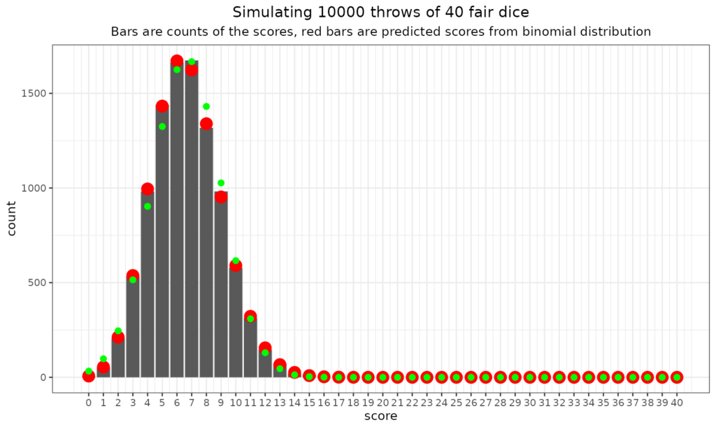
I’ve superimposed the Gaussian probabilities of those scores from zero to 40 based on the observed mean score (6.64) and SD (2.37). The fit is clearly not perfect but it can be seen that the two distributions are getting more similar. This is a phenomenon of the “Central Limit Theorem” (simplifying a bit). This says that as you take the mean of increasing numbers of scores the distribution of those means will get nearer and nearer to Gaussian. This is true pretty much regardless of the distribution of those scores. That’s a bit of a digression and there’s another dice related example of this in the entry for the Gaussian distribution but that example takes the simple scores (i.e. 1 to 6), not the number of sixes. This phenomenon is one reason why the Gaussian distribution not entirely unreasonably underpins classical “parametric statistics”.
Try also #
Distributions
Statistical tests, inferential testing
Estimation
Confidence intervals
Multiple tests problem
Gaussian (“Normal”) distribution
Central limit theorem
Parametric statistics
Chapters #
This doesn’t come directly into any chapter in the book but the logic of distributions, of the binomial distribution and others underpins things in Chapters 5 to 8.
Online resources #
Nothing really useful at this point
Dates #
First created 18.xi.23, links updated 20.xi.23.

