This is the famous “bell shaped curve” which maps the probability of a score as this.

Why does this matter? The simple answer is that if you have a continuous variable, in theory one that can take any value between minus infinity and plus infinity, then if the distribution of its values is Gaussian the maths of working with it is easier than for most other distributions.
That’s a fair but pretty simplified summary. The details are a fairly long story and I try to spell it out next. However, unless you want either to have a much stronger grip of statistics or are just intrigued by the history and elegance of the issues, you can safely skip the details though the links may be useful.
Details #
So what is this? It’s as “probability density function” for a continuous variable which can take values from -infinity to +infinity but has maximum probability at the centre (zero for the “standard Normal” distribution, i.e. halfway between -infinity and +infinity). So it’s a pretty hypothetical thing, why on earth is it generally called “Normal”? Why does it matter?
With others I prefer to call it the Gaussian distribution to avoid this word “Normal” (and please not “normal”: it’s not) and because Carl Friedrich Gauss has one (of several) good claims to have recognised its importance in 1823 (see https://en.wikipedia.org/wiki/Normal_distribution#History for a lovely short summary of the actual history). That points out that de Moivre started its recognition a good 80+ years earlier and Laplace took that further in between the two. The Gaussian distribution matters because it makes possible the whole of “parametric statistics” which, until recent developments in computer power, underpinned the explosion of statistics through the 20th Century.
Although it’s not actually something we see a lot in therapy data, can arise from things as simple as tossing dice. Hang on, didn’t I use tossing a die as an example of a uniform distribution (with observed scores of 1, 2, 3, 4, 5 and 6 equally likely if it’s a fair die). How does that discrete (it only takes six values) uniform distribution get to the bell shaped curve above?
Well, if I tossed six dice repeatedly clearly each time I will get scores between 6 and 36. Here’s the theoretical distribution of scores for that game.

The only actual possible scores are the points but it can be seen that the probability distribution of the possible scores is now far from uniform and is starting to look a bit like this famous bell. Here’s the nearest fit of that Gaussian bell to those probabilities added in green.
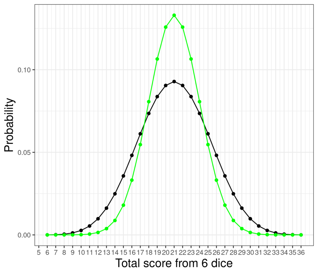
They are clearly different but it can be seen that the score is starting to show a distribution not unlike the Gaussian. Here are the distributions of scores for throwing a single die through to throwing eight.
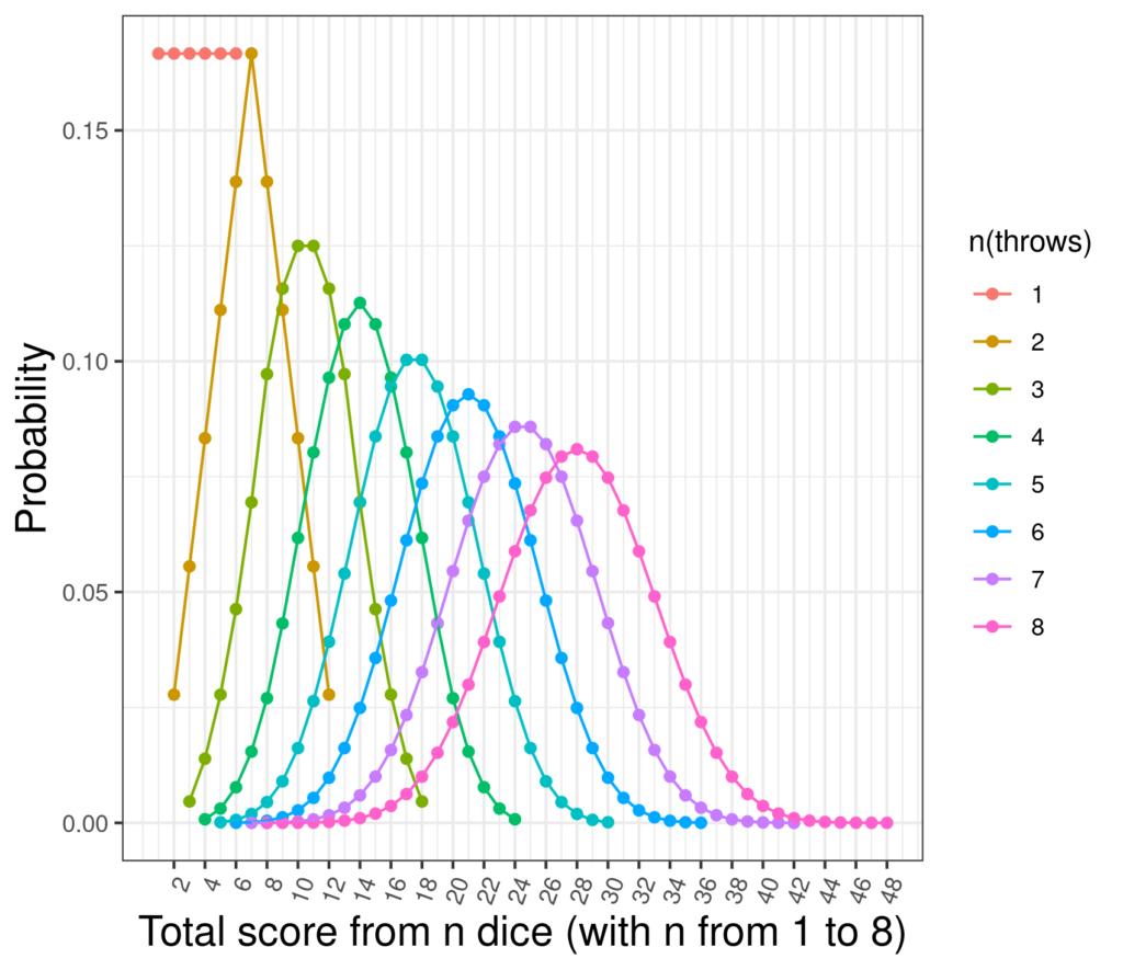
Throwing just one die creates that uniform/flat distribution with each possible score from 1 to 6 equiprobable (at probability 1/6 of course). Two dice creates the inverted v-shaped distribution but by the point at which we are looking at scores of eight dice the distribution is looking much more like a Gaussian (and the score range has moved up to be from 8 to 48 of course).
This is part of what led to the Gaussian distribution being called “normal” or “Normal”: as numbers from (almost any) distribution are summed their distribution tends to the Gaussian. This makes it a particularly plausible model for distributions of “error”. A fact about the Gaussian distribution is that the particular set of scores is always defined by just two “parameters”: the population mean score and the population standard deviation. The so called “standard Gaussian” at the top of this page has mean zero and standard deviation one. Here are two different Gaussians perhaps representing scores on a measure for a help-seeking (HS) and a non-help-seeking (NHS) population.
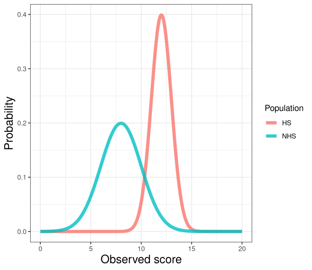
Here the non-help-seeking population has mean 8 and SD 2 and the help-seeking population has mean 12 and SD 1. The smaller SD for the help-seeking population gives it the sharper, thinner shape but the two shapes are the same: if you shifted and stretched the help-seeking curve you could make it fit exactly on the non-help-seeking. Likewise, if you shifted the non-help-seeking curve to the right and squashed it it could fit exactly on the help-seeking curve.
This means that statisticians, mostly through the 20th Century, could work out many ways of exploring data to see if things looked non-random, systematic, based on assumptions about this famous distribution: “parametric statistical methods” so-called because just those two parameters are needed to describe different Gaussian distributions.
If you have reached the end of this and think “I (still) don’t get it!” then I’m sorry but … don’t worry. It really won’t stop you thinking sensibly about data as we have largely moved on from needing to think of things as Gaussian (when generally they are not). It’s just still around in many papers and textbooks.
Try also #
Anderson-Darling test
Arithmetic mean
Binomial distribution
Cramer-von Mises test
Distribution
Distribution tests (“tests of fit to a distribution”)
Error
Histogram
Hypothesis testing, see Inferential testing, “tests”
Kolmogorov-Smirnov test
Parametric statistics
Probability
Shapiro-Francia test
Shapiro-Wilk test
Standard deviation
Statistical tests, see Inferential testing, “tests”
Uniform distribution
Variance
Chapters #
Mostly 5, 7 and 8.
Online resources #
My Rblog posts:
* Explore distributions with plots
* Tests of fit to Gaussian distribution
* Kolmogorov-Smirnov test
My shiny apps:
* App creating samples from Gaussian distribution showing histogram, ecdf and qqplot.
* You can generate samples from distributions using my shiny app: https://shiny.psyctc.org/apps/Create_univariate_data/. At the moment it only creates Gaussian and uniform distributions but more distributions may follow. You can download the data or copy and paste it to other apps.
* You could then paste the data into another app: https://shiny.psyctc.org/apps/ECDFplot/ to get a sense of how your samples change was you change the size or the population parameters (mean and SD for the Gaussian; minimum and maximum for the uniform distribution).
Dates #
Created 5.iii.24, last update 14.i.25.

