I’ve been putting this off! It’s actually quite a basic idea but it covers a lot of complexities and I think they’ll need to be spread across other entries in the glossary but also materials in the Rblog that will provide illustrations for the various related ideas. In turn I will add new shiny apps to my shiny collection that will compute distribution statistics given data. It’s going to be quite a job of work!!
Details #
The basic idea is about scatter. If you only have one observation you have no dispersion, no scatter. Let’s say your variable is the ages of your clients and you start collecting this with your first client who turns out to be aged 27. Now when your second client arrives you have two observations: you have a sort of sample. (More strictly, you have started a dataset, a census of your clients’ ages. If you regard the clients arriving as a sample of the possible clients who might come to you then you do have a sample but I recommend avoiding that word as it can create implications of random sampling from definable populations.) If the second client is also aged 27 you do can have a dispersion statistic but, however you measure it, your dispersion is zero; if the second client is some other age you are starting to have a sample statistic describing the dispersion. That descriptive statistic could be one of a number but variance, or its square root: standard deviation, is the most common. More on that separately.
As you get to say 20 clients you might have a dataset like this (ordered by age not chronological arrival):
18, 18, 18, 19, 19, 19, 20, 20, 20, 21, 23, 23, 24, 24, 24, 25, 27, 28, 30, 31.
However, you might have a dataset like this:
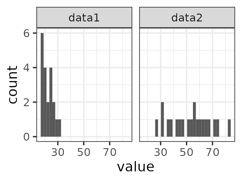
27, 31, 32, 35, 37, 42, 44, 47, 51, 53, 55, 56, 59, 60, 63, 65, 68, 71, 75, 83.
These are clearly rather different distributions, they have different means (22.6 and 52.7 respectively) but they also have very different dispersion values, the variances are 16.4 and 247.2 (SD values 4.0 and 15.7). The first might have come from a student counselling service the second from a private counselling practice. Here are side by side histograms of those data.
One of the key things about acquiring a statistical viewpoint on any data is to start to be interested in dispersion and in the ideas of simplifying descriptions of datasets in terms of two things:
* their central location (typically their mean or median) and
* their dispersion (typically their variance), and beyond those two:
* the shape of a distribution.
The key thing is not so much to know the formula for the mean or median and the variance or SD but to have a sense both of how these can be very useful simplifications that help us handle and understand large datasets. Going with that basic idea is to start to see datasets both in terms of summary numbers but also graphically, to have a sense of the plots that help us see distributions and understand how sometimes too much faith in simple numerical descriptors can mislead us.
Try also #
Mean Absolute Deviation (MAD)
Root Mean Square (RMS) (deviation/dispersion)
Standard deviation (SD)
Variance: introduction
Variance: computation and bias
Chapters #
These ideas really run right through the book but surface most specifically in Chapters 5 and 8.
Online resources #
A good starting point is my shiny app to show sample statistics, histogram, ecdf and qqplot for samples from Gaussian population. You can play with different values of the SD there to get a sense of varying the dispersion of a distribution.
Dates #
First created 11.iii.24, tweaks 13.iii.24.

