This follows on from the introduction to variance. Best to read that first if you’re new to the idea.
Variance, with its related statistic, the standard deviation, which is just the square root of variance, is the most commonly used measure of dispersion across a set of values for a variable. Here’s a tiny dataset of three observations to help explain how the variance is computed.
| wdt_ID | ID | x | mean | discrep | discrepSq |
|---|---|---|---|---|---|
| 1 | 1 | 1 | 6 | -5 | 25 |
| 2 | 2 | 7 | 6 | 1 | 1 |
| 3 | 3 | 10 | 6 | 4 | 16 |
| 4 | Sum: | 18 | 18 | 0 | 42 |
| 5 | Mean: | 6 | 6 | 0 | 14 |
So that shows three observations, values 1, 7 and 10. Their mean is 6 and the discrep column shows the difference between each observation and that mean (-5, 1 and 4) and the final column shows the square of that difference. The two last rows show the sum of the original variable and those computed variables and then their means. In that mean row the fact that the mean of the observations is 6 and that the mean of the means is 6 too and that the mean of the discrepancies from the mean is zero are all just reassuring us that the calculations were done correctly. The last value, 14 is the variance: the mean of the squared differences from the mean.
Here is the same as a plot.
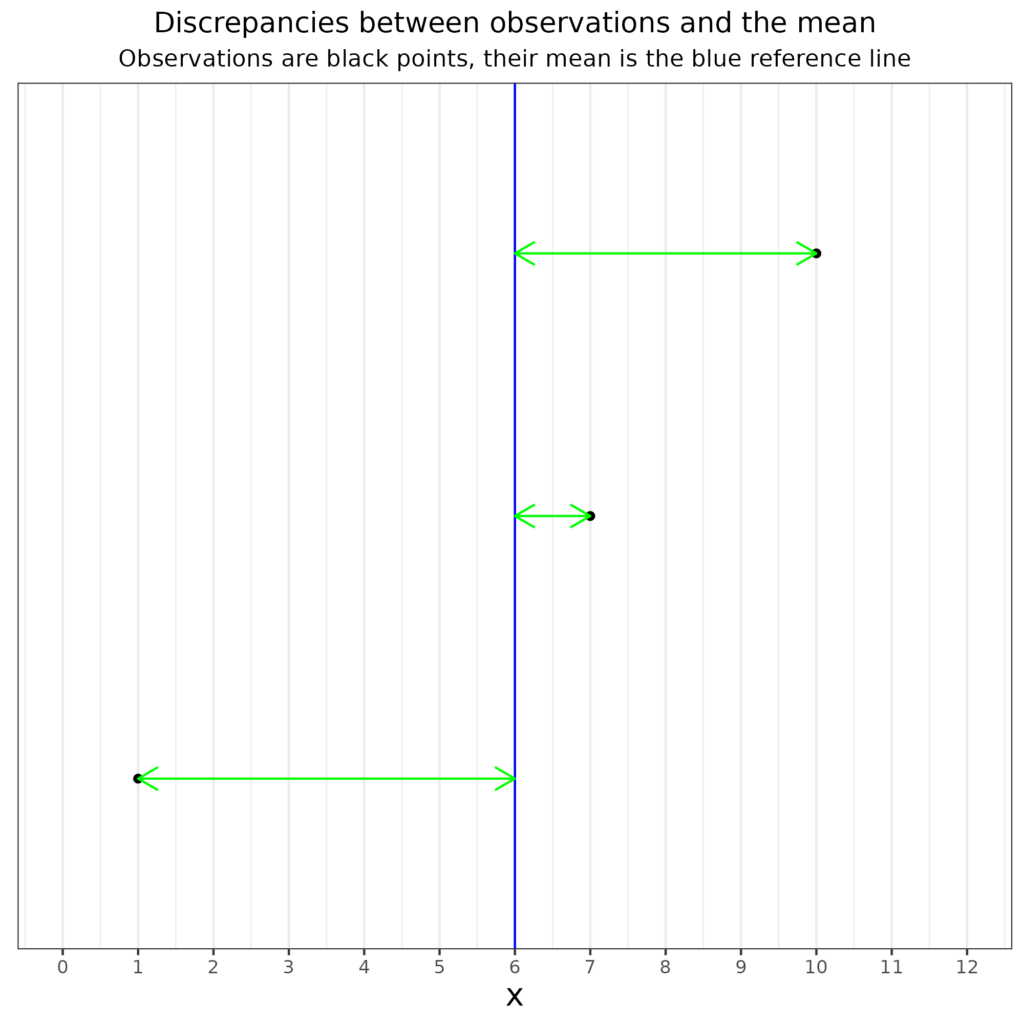
So the variance is the mean of the square of those discrepancies (the lengths of those green arrows).
But there’s a gotcha which I think belongs in details. Read on.
Details #
There are two bits of detail: bias and scale. The first matters for small samples and the second is almost never noted so I think you can probably ignore it!
Bias #
This is all about the sample/population issue. If you are only interested in the discrepancy of your data then that mean of the squared discrepancies from the mean of the observations is all you need. However, if you are interested generalising from your observations, i.e. (for our purposes) treating them as a sample from a population whose unknown variance you are estimating then we hit a snag: in statistical terms the simple variance computed as that mean is a biased estimator of the population variance. It will systematically underestimate the correct population value. This bias is removed if instead of using the mean, i.e. using the sum of the squared discrepancies from the mean divided by the number of observations n we divide by n – 1.
For those who like equations, here is the formula for the variance of a set of data, not treating it as an estimate of a population value but as a census, i.e. a complete ascertainment of the data in that population. Statistics textbooks refer to this as a “population variance” which is technically correct as it’s not an estimate of a population variance. However, I do think that’s confusing for most of us!
$$s^2 = \frac{\sum (x – \bar{x})^2}{n}$$
Where:
\(\sigma^2\) is the population variance, i.e. the variance of the data in that dataset.
\(x\) is the value of a particular observation in the population, i.e. in that dataset.
\(\mu\) is the arithmetic mean of the population, of the dataset values!
\(N\) is the number of observations in the population/dataset.
Here is the formula for the estimate of the population variance with that crucial change to the denominator from n to n – 1.
$$s^2 = \frac{\sum (x – \bar{x})^2}{n-1}$$
Where:
\(\sigma^2\) is now the estimate of the population variance, in statistics textbooks the sample variance.
\(x\) is the value of a particular observation in the population.
\(\mu\) is the arithmetic mean of the observations in the sample.
\(N\) is the number of observations in the sample.
This bias means that if you have a dataset in which the mean square deviations from the mean is 5 that is your “population” variance but the corrected estimate of the population variance, allowing for the bias is like this:
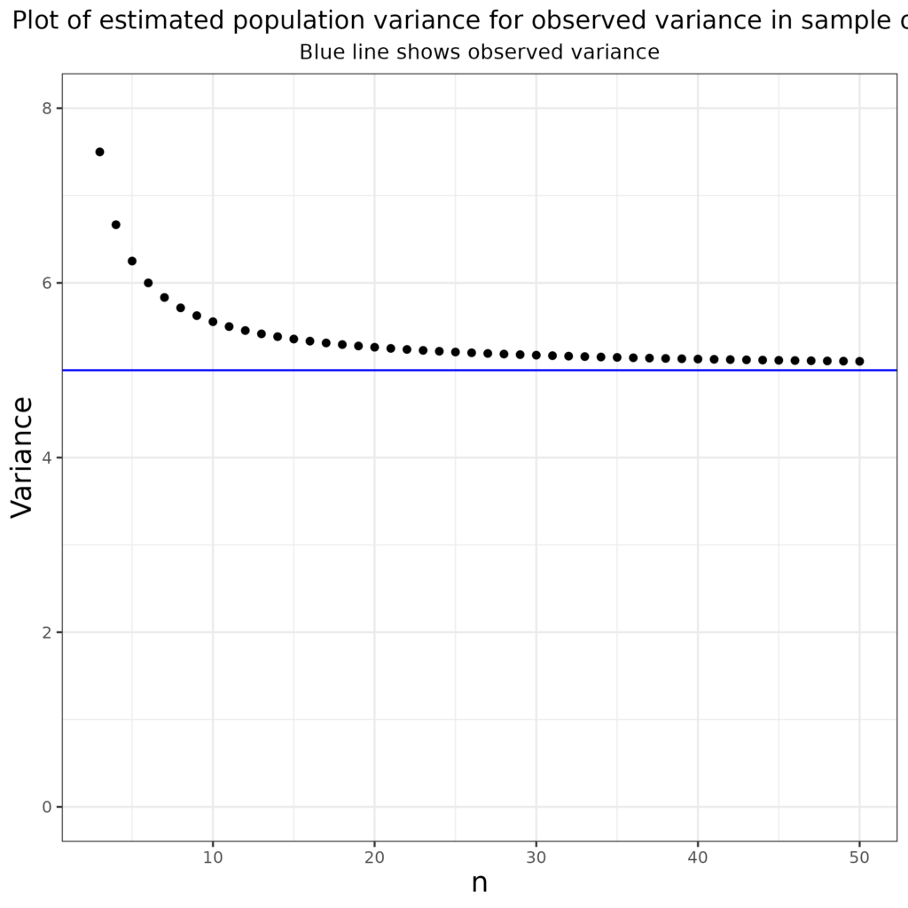
That shows that it’s considerably larger than your observed variance with a (silly) dataset size of 3, actually your best estimate is \(\frac{n}{n-1}\) times your observed value of 5, i.e. 1.5*5 = 7.5.
Here’s a more interesting demonstration of the issue. I simulated 1,000 samples from a population with a Gaussian distribution and variance 5 for a variety of sample sizes from 3 to 50.
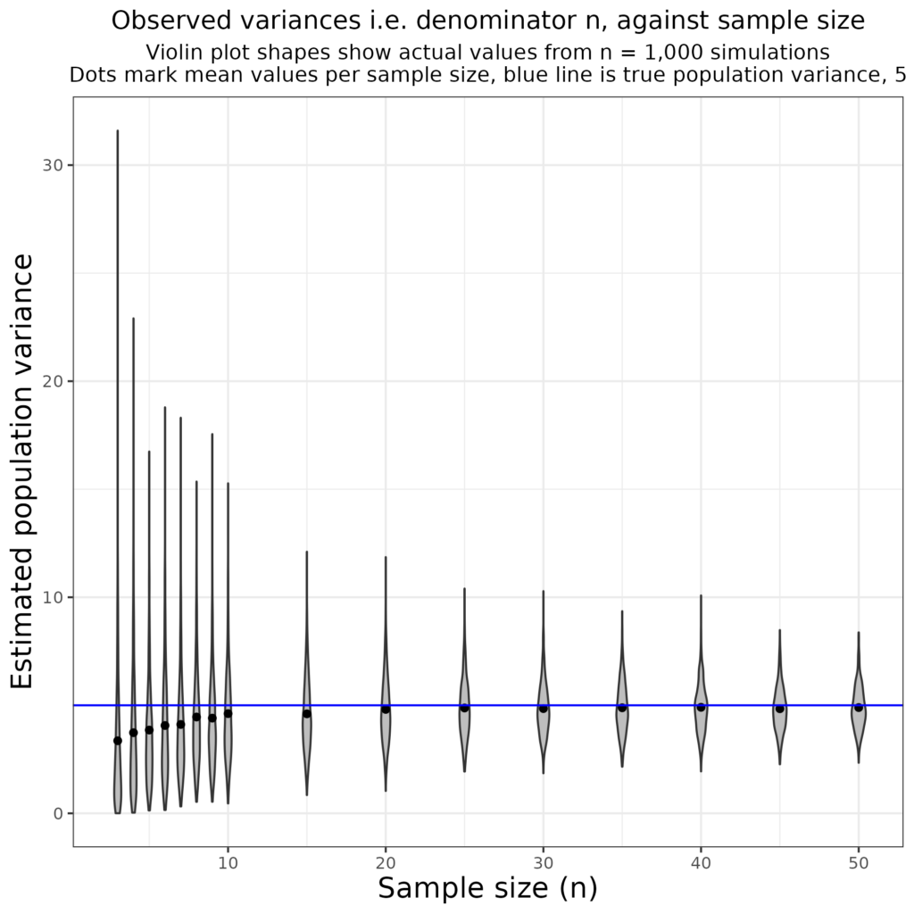
That shows clearly that the simple dataset variances underestimate the known population variance of 5 though the bias decreases as the dataset size, n, increases.
This shows the same simulation but using the unbiased variance estimate with the denominator n – 1.
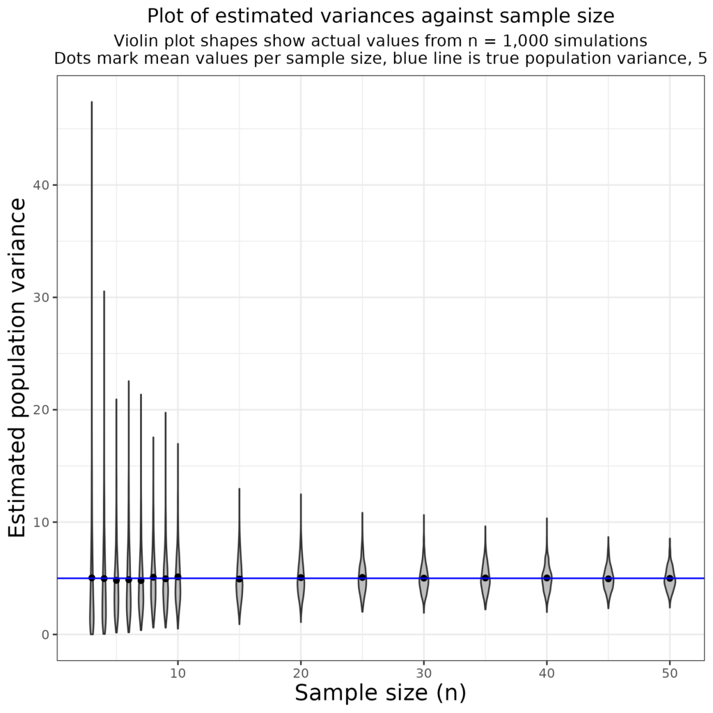
We can see that the use of the n – 1 denominator removes the bias and gives estimates of the population that are always close to 5. Of course, it also shows how the distribution of the variance estimates gets tighter as n increases and the shapes of the “violins” show that at small n the shape of that distribution is very much positively skew and not at all Gaussian but that it appears to be getting closer to symmetrical and perhaps to Gaussian as the n increases. But now I am really getting into esoterica for the purposes of ordinary MH/WB/therapy data.
Scale #
The scale of any variance is the square of the scale of the observations so if those were ages in years the variance is scaled in years squared, if they were scores on some measure then the variance is scaled in the square of that score. I can’t see that I’ve ever seen this noted in publications. It does mean that the scale of its square root is the scale of the original observations so the scale of the SD is the scale of the original observations which is a reason why statistical tests often use the variance but why generally see SD quoted as a descriptive statistic for dispersion rather than the variance.
Try also #
Bias
Distributions
Covariance
Gaussian distribution
Square root
Standard deviation (SD)
Variance: introduction
Chapters #
These issues underpin the statistics in the background of Chapter 5 but we kept them out of the book.
Online resources #
The code for the plots and simulation are at:
* https://www.psyctc.org/Rblog/posts/2021-11-09-ombookglossary/#plot-for-glossary-entry-about-square-root and
* https://www.psyctc.org/Rblog/posts/2021-11-09-ombookglossary/#variance-glossary-entry
Dates #
First created 12-13.iii.24.

