This is one of three different “seven number” summaries of the distribution of a set of scores which are all extensions of the five point summary (minimum, lower quartile, median, upper quartile and maximum to save you clicking through!)
Details #
This seven number summary splits a distribution into eight score ranges. The cutting points here are “2.15%”, “8.87%”, “25%”, “50%”, “75%”, “91.13%” and “97.85%”, so as proportions those are 0.0215, 0.0887, 0.25, 0.5, 0.75, 0.9113 and 0.9785. The logic is that if the distribution is Gaussian those points would be about equally spaced across the range of the scores. Apparently it was associated with a box plot with extra “whiskers”. Here’s an example for 5,000 values of a Gaussian distribution with mean 1.0 and SD 1 and the cubes of those numbers transformed to re-centre then on 1.00 and to have an SD again of 1.0.
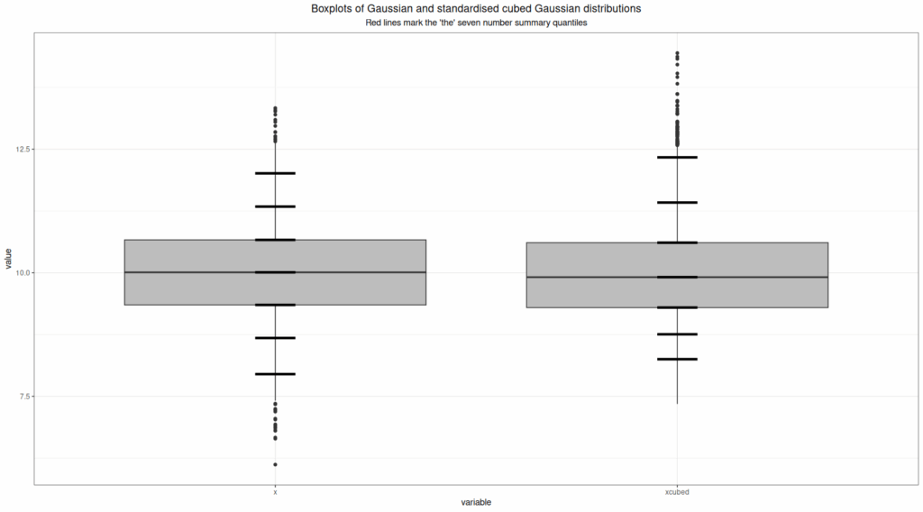
It can be seen there that three central cutting points (lower quartile, median and upper quartile) are almost the same for the Gaussian distribution on the left and the non-Gaussian distribution on the right and that those look pretty equally spaced. It can also be seen that the additional four “whiskers” above and below the box that form this seven number summary are not equally spaced. It can be argued that this makes this a useful enhancement to the five number summary and ordinary boxplot. However, here are the histograms of the same data with the closest fitting Gaussian distributions as red density lines.
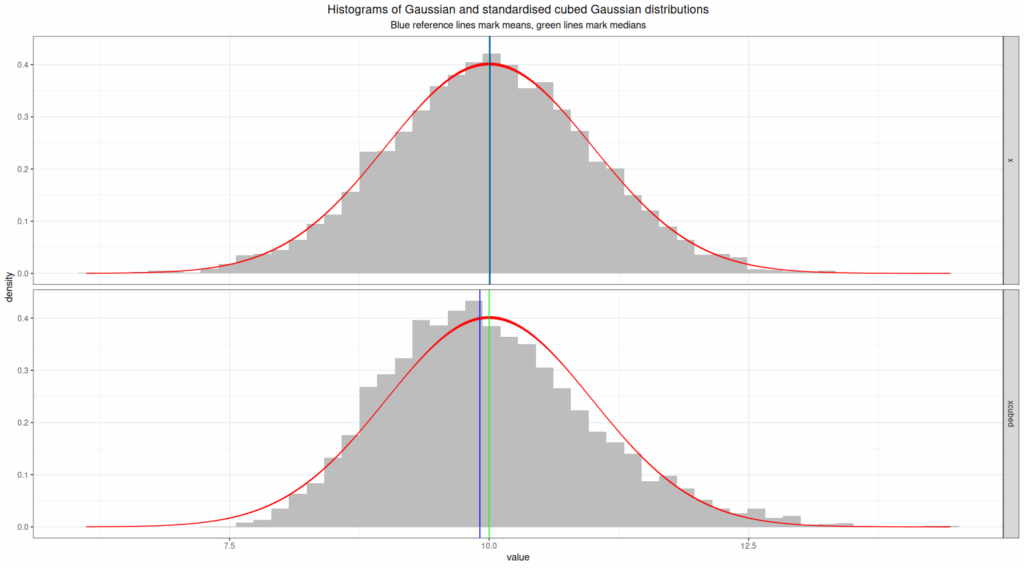
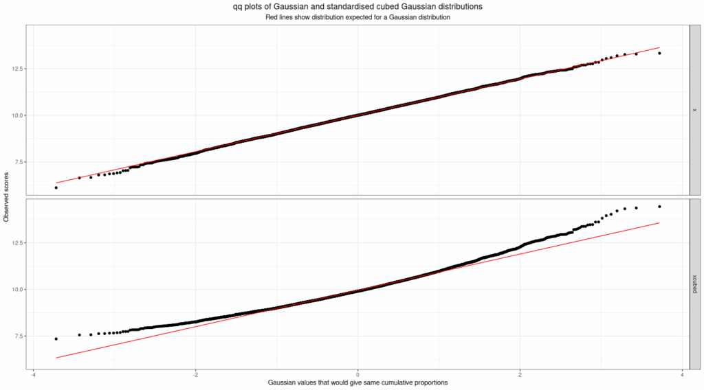
I think that’s a much better way to see the distribution of the data and to see that the second dataset clearly doesn’t fit a Gaussian distribution whereas the first looks like very close fit to Gaussian. The qq plot is an even better way to detect deviation from Gaussian distribution by eyeballing a plot as this next plot shows.
Of course if you really want this there are good null hypothesis tests that test the fit of a set of data to a Gaussian distribution. Equally, the preoccupation with whether or not distributions are Gaussian or not is essentially a historical one now we have bootstrap methods and, I hope, are finally losing the overvaluation of the whole NHST (Null Hypothesis Significance Testing) paradigm which was so linked with “parametric tests” with their assumptions of Gaussian population distributions.
Summary #
I think we can forget this seven number summary!
Try also #
- Bootstrap, bootstrapping and …
- Bootstrap method (with more detail)
- Bowley’s seven-figure summary
- Distribution and …
- Distribution shape
- Five point summary
- Gaussian (“Normal”) distribution
- Null hypothesis significance testing paradigm (NHST)
- Percentiles
- Quantiles
- Quartiles
- Seven point summaries
- Test of fit to a distribution
- Tukey’s seven-number summary
Chapters #
Not covered in the OMbook.
Online resources #
One of my shiny apps: ECDF plot with quantiles and CIs for quantiles is pertinent in the unlikely event that you ever want to get any of these seven point splits of your data with their confidence intervals!
In my Rblog there are posts on exploring distributions with plots, tests of fit to Gaussian distribution and on the Kolmogorov-Smirnov test which is a very bad test of fit if testing fit to Gaussian distribution.
Dates #
First created 3.v.25

